11.4 Variance and standard deviation | Statistics

11.4 Variance and standard deviation (EMBK8)

Measures of central tendency (mean, median and mode) provide information on the data values at the centre of the data set. Measures of dispersion (quartiles, percentiles, ranges) provide information on the spread of the data around the centre. In this section we will look at two more measures of dispersion called the variance and the standard deviation.

Video: 23CV

Variance (EMBK9)

Variance

Let a population consist of \(n\) elements, \(\{x_1; x_2; \ldots; x_n\}\). Write the mean of the data as \(\overline{x}\).

The variance of the data is the average squared distance between the mean and each data value. \[\sigma^2 = \frac{\sum_{i=1}^n \left(x_i - \overline{x}\right)^2}{n}\]

The variance is written as \(\sigma^2\). It might seem strange that it is written in squared form, but you will see why soon when we discuss the standard deviation.

The variance has the following properties.

It is never negative since every term in the variance sum is squared and therefore either positive or zero.
It has squared units. For example, the variance of a set of heights measured in centimetres will be given in centimeters squared. Since the population variance is squared, it is not directly comparable with the mean or the data themselves. In the next section we will describe a different measure of dispersion, the standard deviation, which has the same units as the data.

Worked example 10: Variance

You flip a coin \(\text{100}\) times and it lands on heads \(\text{44}\) times. You then use the same coin and do another \(\text{100}\) flips. This time in lands on heads \(\text{49}\) times. You repeat this experiment a total of \(\text{10}\) times and get the following results for the number of heads. \[\{44; 49; 52; 62; 53; 48; 54; 49; 46; 51\}\]

Compute the mean and variance of this data set.

Compute the mean

The formula for the mean is \[\overline{x} = \frac{\sum_{i=1}^n x_i}{n}\]

In this case, we sum the data and divide by \(\text{10}\) to get \(\overline{x} = \text{50,8}\).

Compute the variance

The formula for the variance is \[\sigma^2 = \frac{\sum_{i=1}^n \left(x_i - \overline{x}\right)^2}{n}\]

We first subtract the mean from each datum and then square the result.

\(x_i\)	\(\text{44}\)	\(\text{49}\)	\(\text{52}\)	\(\text{62}\)	\(\text{53}\)	\(\text{48}\)	\(\text{54}\)	\(\text{49}\)	\(\text{46}\)	\(\text{51}\)
\(x_i - \overline{x}\)	\(-\text{6,8}\)	\(-\text{1,8}\)	\(\text{1,2}\)	\(\text{11,2}\)	\(\text{2,2}\)	\(-\text{2,8}\)	\(\text{3,2}\)	\(-\text{1,8}\)	\(-\text{4,8}\)	\(\text{0,2}\)
\((x_i - \overline{x})^2\)	\(\text{46,24}\)	\(\text{3,24}\)	\(\text{1,44}\)	\(\text{125,44}\)	\(\text{4,84}\)	\(\text{7,84}\)	\(\text{10,24}\)	\(\text{3,24}\)	\(\text{23,04}\)	\(\text{0,04}\)

The variance is the sum of the last row in this table divided by \(\text{10}\), so \(\sigma^2 = \text{22,56}\).

temp text

Standard deviation (EMBKB)

Since the variance is a squared quantity, it cannot be directly compared to the data values or the mean value of a data set. It is therefore more useful to have a quantity which is the square root of the variance. This quantity is known as the standard deviation.

Standard deviation: Let a population consist of \(n\) elements, \(\{x_1; x_2; \ldots; x_n\}\), with a mean of \(\overline{x}\). The standard deviation of the data is \[\sigma = \sqrt{\frac{\sum_{i=1}^n \left(x_i - \overline{x}\right)^2}{n}}\]

In statistics, the standard deviation is a very common measure of dispersion. Standard deviation measures how spread out the values in a data set are around the mean. More precisely, it is a measure of the average distance between the values of the data in the set and the mean. If the data values are all similar, then the standard deviation will be low (closer to zero). If the data values are highly variable, then the standard variation is high (further from zero).

The standard deviation is always a positive number and is always measured in the same units as the original data. For example, if the data are distance measurements in kilogrammes, the standard deviation will also be measured in kilogrammes.

The mean and the standard deviation of a set of data are usually reported together. In a certain sense, the standard deviation is a natural measure of dispersion if the centre of the data is taken as the mean.

Video: 23CW

Tabulating results

It is often useful to set your data out in a table so that you can apply the formulae easily. Complete the table below to calculate the standard deviation of \(\{\text{57}; \text{53}; \text{58}; \text{65}; \text{48}; \text{50}; \text{66}; \text{51}\}\).

Firstly, remember to calculate the mean, \(\overline{x}\).
Complete the following table.

index: \(i\)	datum: \(x_i\)	deviation: \(x_i - \overline{x}\)	deviation squared: \((x_i - \overline{x})^2\)
\(\text{1}\)	\(\text{57}\)
\(\text{2}\)	\(\text{53}\)
\(\text{3}\)	\(\text{58}\)
\(\text{4}\)	\(\text{65}\)
\(\text{5}\)	\(\text{48}\)
\(\text{6}\)	\(\text{50}\)
\(\text{7}\)	\(\text{66}\)
\(\text{8}\)	\(\text{51}\)
	\(\sum x_i = \ldots\)	\(\sum (x_i - \overline{x}) = \ldots\)	\(\sum (x_i - \overline{x})^2 = \ldots\)

The sum of the deviations is always zero. Why is this? Find out.
Calculate the variance using the completed table.
Then calculate the standard deviation.

Worked example 11: Variance and standard deviation

What is the variance and standard deviation of the possibilities associated with rolling a fair die?

Determine all the possible outcomes

When rolling a fair die, the sample space consists of \(\text{6}\) outcomes. The data set is therefore \(x=\left\{1;2;3;4;5;6\right\}\) and \(n = 6\).

Calculate the mean

The mean is: \begin{align*} \overline{x} &= \frac{1}{6}\left(1+2+3+4+5+6\right) \\ &= \text{3,5} \end{align*}

Calculate the variance

The variance is: \begin{align*} \sigma^2 &= \frac{\sum {\left(x-\overline{x}\right)}^{2}}{n} \\ &= \frac{1}{6}\left(\text{6,25}+\text{2,25}+\text{0,25}+\text{0,25}+\text{2,25}+\text{6,25}\right) \\ &= \text{2,917} \end{align*}

Calculate the standard deviation

The standard deviation is: \begin{align*} \sigma &= \sqrt{\text{2,917}} \\ &= \text{1,708} \end{align*}

temp text

Interpretation and application (EMBKC)

A large standard deviation indicates that the data values are far from the mean and a small standard deviation indicates that they are clustered closely around the mean.

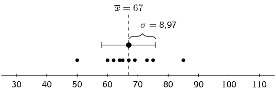
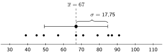
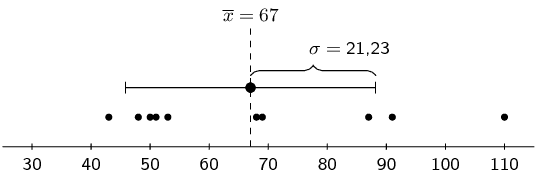
For example, consider the following three data sets: \begin{align*} & \{65; 75; 73; 50; 60; 64; 69; 62; 67; 85\} \\ & \{85; 79; 57; 39; 45; 71; 67; 87; 91; 49\} \\ & \{43; 51; 53; \text{110}; 50; 48; 87; 69; 68; 91\} \end{align*}

Each of these data sets has the same mean, namely \(\text{67}\). However, they have different standard deviations, namely \(\text{8,97}\), \(\text{17,75}\) and \(\text{21,23}\). The following figures show plots of the data sets with the mean and standard deviation indicated on each. You can see how the standard deviation is larger when the data are more spread out.

\(\begin{array}{l@{\quad}r@{\;}l} \text{data:} & \{x_i\} &= \{65; 75; 73; 50; 60; 64; 69; 62; 67; 85\} \\ \text{mean:} & \overline{x} & = 67 \\ \text{standard deviation:} & \sigma &\approx \text{8,97} \end{array}\)

\(\begin{array}{l@{\quad}r@{\;}l} \text{data:} & \{x_i\} &= \{85; 79; 57; 39; 45; 71; 67; 87; 91; 49\} \\ \text{mean:} & \overline{x} & = 67 \\ \text{standard deviation:} & \sigma &\approx \text{17,75} \end{array}\)

\(\begin{array}{l@{\quad}r@{\;}l} \text{data:} & \{x_i\} &= \{43; 51; 53; \text{110}; 50; 48; 87; 69; 68; 91\} \\ \text{mean:} & \overline{x} & = 67 \\ \text{standard deviation:} & \sigma &\approx \text{21,23} \end{array}\)

The standard deviation may also be thought of as a measure of uncertainty. In the physical sciences, for example, the reported standard deviation of a group of repeated measurements represents the precision of those measurements. When deciding whether measurements agree with a theoretical prediction, the standard deviation of those measurements is very important: if the mean of the measurements is too far away from the prediction (with the distance measured in standard deviations), then we consider the measurements as contradicting the prediction. This makes sense since they fall outside the range of values that could reasonably be expected to occur if the prediction were correct.

Variance and standard deviation

Textbook Exercise 11.4

Bridget surveyed the price of petrol at petrol stations in Cape Town and Durban. The data, in rands per litre, are given below.

Cape Town	\(\text{3,96}\)	\(\text{3,76}\)	\(\text{4,00}\)	\(\text{3,91}\)	\(\text{3,69}\)	\(\text{3,72}\)
Durban	\(\text{3,97}\)	\(\text{3,81}\)	\(\text{3,52}\)	\(\text{4,08}\)	\(\text{3,88}\)	\(\text{3,68}\)

Find the mean price in each city and then state which city has the lower mean.

Cape Town: \(\text{3,84}\). Durban: \(\text{3,82}\). Durban has the lower mean.

Find the standard deviation of each city's prices.

Standard deviation: \[\sigma = \sqrt{\frac{\sum {\left(x-\overline{x}\right)}^{2}}{n}}\]

For Cape Town: \begin{align*} \sigma &= \sqrt{\frac{\sum {\left(x-(\text{3,84})\right)}^{2}}{\text{6}}} \\ &= \sqrt{\frac{\text{0,0882}}{\text{6}}} \\ &= \sqrt{\text{0,0147}} \\ &\approx \text{0,121} \end{align*}

For Durban: \begin{align*} \sigma &= \sqrt{\frac{\sum {\left(x-(\text{3,82}\dot{3})\right)}^{2}}{\text{6}}} \\ &= \sqrt{\frac{\text{0,20}\dot{3}}{\text{6}}} \\ &= \sqrt{\text{0,033}\dot{8}} \\ &\approx \text{0,184} \end{align*}

Which city has the more consistently priced petrol? Give reasons for your answer.

The standard deviation of Cape Town's prices is lower than that of Durban's. That means that Cape Town has more consistent (less variable) prices than Durban.

Compute the mean and variance of the following set of values.

\(\text{150}\) ; \(\text{300}\) ; \(\text{250}\) ; \(\text{270}\) ; \(\text{130}\) ; \(\text{80}\) ; \(\text{700}\) ; \(\text{500}\) ; \(\text{200}\) ; \(\text{220}\) ; \(\text{110}\) ; \(\text{320}\) ; \(\text{420}\) ; \(\text{140}\)

Mean = \(\text{270,7}\). Variance = \(\text{27 435,2}\).

Compute the mean and variance of the following set of values.

\(-\text{6,9}\) ; \(-\text{17,3}\) ; \(\text{18,1}\) ; \(\text{1,5}\) ; \(\text{8,1}\) ; \(\text{9,6}\) ; \(-\text{13,1}\) ; \(-\text{14,0}\) ; \(\text{10,5}\) ; \(-\text{14,8}\) ; \(-\text{6,5}\) ; \(\text{1,4}\)

Mean = \(-\text{1,95}\). Variance = \(\text{127,5}\).

Calculate the mean time.

\(\overline{x} = \text{10,4}\)

Calculate the standard deviation for the data.

\(\sigma = \text{0,27}\)

How many of the athletes' times are more than one standard deviation away from the mean?

The mean is \(\text{10,4}\) and the standard deviation is \(\text{0,27}\). Therefore the interval containing all values that are one standard deviation from the mean is \(\left[\text{10,4}-\text{0,27} ; \text{10,4}+\text{0,27}\right] = \left[\text{10,13} ; \text{10,67}\right]\). We are asked how many values are further than one standard deviation from the mean, meaning outside the interval. There are \(\text{3}\) values from the data set outside the interval.

The following data set has a mean of \(\text{14,7}\) and a variance of \(\text{10,01}\).

\[\text{18}\ ;\ \text{11}\ ;\ \text{12}\ ;\ a\ ;\ \text{16}\ ;\ \text{11}\ ;\ \text{19}\ ;\ \text{14}\ ;\ b\ ;\ \text{13}\]

Compute the values of \(a\) and \(b\).

From the formula of the mean we have \begin{align*} \text{14,7} &= \frac{\text{114} + a + b}{10} \\ \therefore a + b &= \text{147} - \text{114} \\ \therefore a &= 33-b \end{align*}

From the formula of the variance we have \begin{align*} \sigma^2 &= \frac{\sum_{i=1}^n (x_i-\overline{x})^2}{n} \\ \therefore \text{10,01} &= \frac{\text{69,12} + (a-\text{14,7})^2 + (b-\text{14,7})^2}{10} \end{align*}

Substitute \(a = 33-b\) into this equation to get \begin{align*} \text{10,01} &= \frac{\text{69,12} + (\text{18,3}-b)^2 + (b-\text{14,7})^2}{10} \\ \therefore \text{100,1} &= 2b^2 - \text{66}b + \text{620,1} \\ \therefore 0 &= b^2 - \text{33}b + \text{260} \\ &= (b-13)(b-20) \end{align*} Therefore \(b = 13\) or \(b = 20\).

Since \(a = 33-b\) we have \(a = 20\) or \(a = 13\). So, the two unknown values in the data set are \(\text{13}\) and \(\text{20}\).

We do not know which of these is \(a\) and which is \(b\) since the mean and variance tell us nothing about the order of the data.

11.3 Ogives

Table of Contents

11.5 Symmetric and skewed data