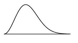
A data set with this distribution:
|
Previous
End of chapter exercises
|
Next
9.2 Curve fitting
|
Measures of central tendency:
Provide information on the data values at the centre of the data set.
The median is the middle value of an ordered data set. To find the median, we first sort the data in ascending or descending order and then pick out the value in the middle of the sorted list. If the middle is in between two values, the median is the average of those two values.
Measures of dispersion:
Tell us how spread out a data set is. If a measure of dispersion is small, the data are clustered in a small region. If a measure of dispersion is large, the data are spread out over a large region.
The range is the difference between the maximum and minimum values in the data set.
The inter-quartile range is the difference between the first and third quartiles of the data set. The quartiles are computed in a similar way to the median. The median is halfway into the ordered data set and is sometimes also called the second quartile. The first quartile is one quarter of the way into the ordered data set, whereas the third quartile is three quarters of the way into the ordered data set.
If you begin numbering your ordered data set with the number 1, the formulae for the location of each quartile are as follows: \begin{align*} \text{Location of } Q_{1} & = \frac{1}{4}(n-1)+1 \\ \text{Location of } Q_{2} & = \frac{1}{2}(n-1)+1 \\ \text{Location of } Q_{3} & = \frac{3}{4}(n-1)+1 \end{align*}
The variance of the data is the average squared distance between the mean and each data value.
The variance of the data is \[\sigma^2 = \frac{\sum\limits_{i=1}^n \left(x_i - \bar{x}\right)^2}{n}\] in a population of \(n\) elements, \(\{x_1; x_2; \ldots; x_n\}\), with a mean of \(\bar{x}\).
The standard deviation measures how spread out the values in a data set are around the mean. More precisely, it is a measure of the average distance between the values of the data in the set and the mean.
The standard deviation of the data is \[\sigma = \sqrt{\frac{\sum\limits_{i=1}^n \left(x_i - \bar{x}\right)^2}{n}}\] in a population of \(n\) elements, \(\{x_1; x_2; \ldots; x_n\}\), with a mean of \(\bar{x}\).
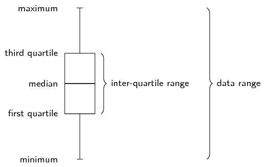
The five number summary combines a measure of central tendency, the median, with measures of dispersion, namely the range and the inter-quartile range. More precisely, the five number summary is written in the following order:
The five number summary is often presented visually using a box and whisker diagram, illustrated below.
Draw a box and whisker diagram for the following data set: \[\text{1,25}\ ;\ \text{1,5}\ ;\ \text{2,5}\ ;\ \text{2,5}\ ;\ \text{3,1}\ ;\ \text{3,2}\ ;\ \text{4,1}\ ;\ \text{4,25}\ ;\ \text{4,75}\ ;\ \text{4,8}\ ;\ \text{4,95}\ ;\ \text{5,1}\]
Since the data set is already ordered, we can read off the minimum as the first value (\(\text{1,25}\)) and the maximum as the last value (\(\text{5,1}\)).
There are \(\text{12}\) values in the data set. We can use the figure below or the formulae to determine where the quartiles are located.

Using the figure above we can see that the median is between the sixth and seventh values. We can confirm this using the formula: \begin{align*} \text{Location of } Q_{2} & = \frac{1}{2}(n-1)+1 \\ &= \frac{1}{2}(11)+1 \\ &=\text{6,5} \end{align*} Therefore, the value of the median is \[\frac{\text{3,2}+\text{4,1}}{2} = \text{3,65}\]
The first quartile lies between the third and fourth values. We can confirm this using the formula: \begin{align*} \text{Location of } Q_{1} & = \frac{1}{4}(n-1)+1 \\ &= \frac{1}{4}(11)+1 \\ &=\text{3,75} \end{align*} Therefore, the value of the first quartile is \[Q_1 = \frac{\text{2,5}+\text{2,5}}{2} = \text{2,5}\]
The third quartile lies between the ninth and tenth values. We can confirm this using the formula: \begin{align*} \text{Location of } Q_{3} & = \frac{3}{4}(n-1)+1 \\ &= \frac{3}{4}(11)+1 \\ &=\text{9,25} \end{align*} Therefore, the value of the third quartile is \[Q_3 = \frac{\text{4,75}+\text{4,8}}{2} = \text{4,775}\]
We now have the five number summary as (\(\text{1,25}\); \(\text{2,5}\); \(\text{3,65}\); \(\text{4,775}\); \(\text{5,1}\)). The box and whisker diagram representing the five number summary is given below.

You flip a coin \(\text{100}\) times and it lands on heads \(\text{44}\) times. You then use the same coin and do another \(\text{100}\) flips. This time in lands on heads \(\text{49}\) times. You repeat this experiment a total of \(\text{10}\) times and get the following results for the number of heads. \[\{44; 49; 52; 62; 53; 48; 54; 49; 46; 51\}\]
For the data set above:
The formula for the mean is \[\overline{x} = \frac{\sum_{i=1}^n x_i}{n}\]
In this case, we sum the data and divide by \(\text{10}\) to get \(\overline{x} = \text{50,8}\).
The formula for the variance is \[\sigma^2 = \frac{\sum_{i=1}^n \left(x_i - \overline{x}\right)^2}{n}\]
We first subtract the mean from each data point and then square the result.
| \(x_i\) | \(\text{44}\) | \(\text{49}\) | \(\text{52}\) | \(\text{62}\) | \(\text{53}\) | \(\text{48}\) | \(\text{54}\) | \(\text{49}\) | \(\text{46}\) | \(\text{51}\) |
| \(x_i - \overline{x}\) | \(-\text{6,8}\) | \(-\text{1,8}\) | \(\text{1,2}\) | \(\text{11,2}\) | \(\text{2,2}\) | \(-\text{2,8}\) | \(\text{3,2}\) | \(-\text{1,8}\) | \(-\text{4,8}\) | \(\text{0,2}\) |
| \((x_i - \overline{x})^2\) | \(\text{46,24}\) | \(\text{3,24}\) | \(\text{1,44}\) | \(\text{125,44}\) | \(\text{4,84}\) | \(\text{7,84}\) | \(\text{10,24}\) | \(\text{3,24}\) | \(\text{23,04}\) | \(\text{0,04}\) |
The variance is the sum of the last row in this table divided by \(\text{10}\), so \(\sigma^2 = \text{22,56}\).
\(\\\)Using the SHARP EL-531VH calculator:
Using your calculator, change the mode from normal to “Stat \(x\) ”. Do this by pressing [2ndF] and then 1. This mode enables you to type in univariate data.
Key in the data, row by row:
|
Enter: |
Press: |
See: |
|
44 |
DATA |
n = \(\text{1}\) |
|
49 |
DATA |
n = \(\text{2}\) |
|
52 |
DATA |
n = \(\text{3}\) |
|
62 |
DATA |
n = \(\text{4}\) |
|
53 |
DATA |
n = \(\text{5}\) |
|
48 |
DATA |
n = \(\text{6}\) |
|
54 |
DATA |
n = \(\text{7}\) |
|
49 |
DATA |
n = \(\text{8}\) |
|
46 |
DATA |
n = \(\text{9}\) |
|
51 |
DATA |
n = \(\text{10}\) |
Note: The [DATA] button is the same as the [M+] button.
Get the value for \(\sigma_{x}\):
|
Press: |
Press: |
See: |
|
RCL |
\(\sigma x\) |
\(\sigma x= \pm\text{4,75}\) |
Using the CASIO \(fx\)-82ZA PLUS calculator:
Switch on the calculator. Press [MODE] and then select STAT by pressing [2]. The following screen will appear:
|
1 |
\(1-VAR\) |
2 |
\(A+BX\) |
|
3 |
\(_+C{X}^{2}\) |
4 |
\(lnX\) |
|
5 |
\(eX\) |
6 |
\(A.B\)\(X\) |
|
7 |
\(A.XB\) |
8 |
\(1/X\) |
Now press [1] for variance and standard deviation. Your screen should look something like this:
|
\(x\) |
|
|
1 |
|
|
2 |
|
|
3 |
Press [44] and then [\(=\)] to enter the first \(x\)-value under \(x\). Then enter the other values in the same way.
|
\(x\) |
|
|
1 |
44 |
|
2 |
49 |
|
3 |
52 |
Then press [AC]. The screen clears but the data remains stored.
Now press [SHIFT][1] to get the stats computations screen shown below.
|
1: |
Type |
2: |
Data |
|
3: |
Sum |
4: |
Var |
|
5: |
MinMax |
Choose variance by pressing [4].
|
1: |
n |
2: |
\(\bar{x}\) |
|
3: |
\(\sigma x\) |
4: |
s\(x\) |
Get the value for \(\sigma_{x}\):
Press [3] and [=] to get the value of \(\sigma x\)
\(\therefore \sigma_{x}=\pm\text{4,75} \text{ and } {\sigma_{x}}^{2}=(\text{4,75})^{2} = \text{22,56}\)Last year you learnt about three shapes of data distribution: symmetric, left skewed and right skewed.
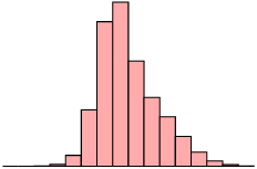
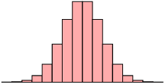
A symmetric distribution is one where the left and right hand sides of the distribution are roughly equally balanced around the mean. The histogram below shows a typical symmetric distribution.
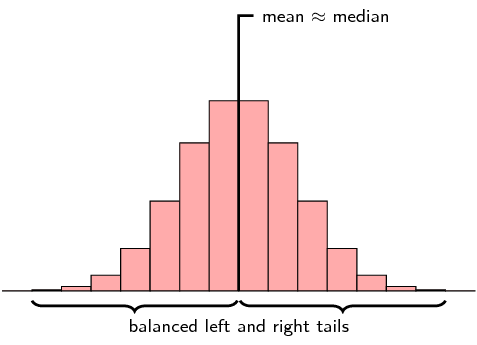
For symmetric distributions, the mean is approximately equal to the median and the left and right tails are equally balanced, meaning that they have about the same length.
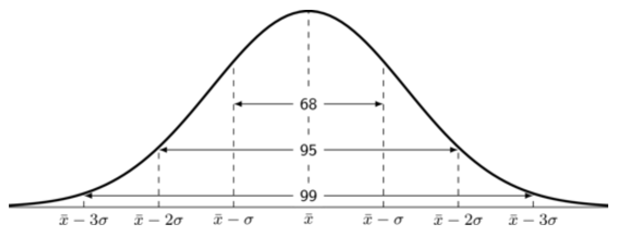
If large numbers of data are collected from a population, the graph will often have a bell shape. If the data was, say, examination results, a few learners usually get very high marks, a few very low marks and most get a mark in the middle range. This is a common type of symmetric data known as a normal distribution. We say a distribution is normal if
the mean, median and mode are equal.
it is symmetric around the mean.
\(\text{68}\%\) of the sample lies within one standard deviation of the mean, \(\text{95}\%\) within two standard deviations and \(\text{99}\%\) within three standard deviations of the mean.
What happens if the test was very easy or very difficult? Then the distribution may not be symmetrical. If extremely high or extremely low scores are added to a distribution, then the mean and median tend to shift towards these scores and the curve becomes skewed.
If the test was very difficult, the mean and median scores are shifted to the left. In this case, we say the distribution is positively skewed, or skewed right.
A distribution that is skewed right has the following characteristics:
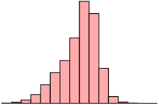
If the test was very easy, then many learners would get high scores, and the mean and median of the distribution would be shifted to the right. We say the distribution is negatively skewed, or skewed left.
A distribution that is skewed right has the following characteristics:
The table below summarises the different categories visually.
| Skewed right (positive) | Symmetric | Skewed left (negative) |
 |
 |
 |
 |
 |
 |
| mean \(>\) median | mean \(\approx\) median | mean \(<\) median |
Three Matric classes wrote a Mathematics test. The test is out of \(\text{40}\) marks and each class has \(\text{21}\) learners. The results of the test are shown in the table below:
| Gr. 12A | Gr. 12B | Gr. 12C |
| \(\text{4}\) | \(\text{4}\) | \(\text{4}\) |
| \(\text{8}\) | \(\text{12}\) | \(\text{6}\) |
| \(\text{8}\) | \(\text{16}\) | \(\text{6}\) |
| \(\text{12}\) | \(\text{16}\) | \(\text{10}\) |
| \(\text{12}\) | \(\text{16}\) | \(\text{14}\) |
| \(\text{12}\) | \(\text{16}\) | \(\text{14}\) |
| \(\text{12}\) | \(\text{16}\) | \(\text{16}\) |
| \(\text{16}\) | \(\text{20}\) | \(\text{16}\) |
| \(\text{16}\) | \(\text{20}\) | \(\text{18}\) |
| \(\text{16}\) | \(\text{28}\) | \(\text{18}\) |
| \(\text{16}\) | \(\text{32}\) | \(\text{21}\) |
| \(\text{32}\) | \(\text{32}\) | \(\text{24}\) |
| \(\text{32}\) | \(\text{32}\) | \(\text{24}\) |
| \(\text{32}\) | \(\text{32}\) | \(\text{24}\) |
| \(\text{36}\) | \(\text{36}\) | \(\text{28}\) |
| \(\text{36}\) | \(\text{36}\) | \(\text{30}\) |
| \(\text{36}\) | \(\text{36}\) | \(\text{32}\) |
| \(\text{40}\) | \(\text{36}\) | \(\text{36}\) |
| \(\text{40}\) | \(\text{40}\) | \(\text{36}\) |
| \(\text{40}\) | \(\text{40}\) | \(\text{36}\) |
| \(\text{40}\) | \(\text{40}\) | \(\text{40}\) |
First, we order the data from smallest to largest. This has already been done for us. Then, we divide our data into quartiles:

The minimum of each data set is \(\text{4}\). The maximum of each data set is \(\text{40}\).
Since there are \(\text{21}\) values in the data set, the median lies on the eleventh mark, making it equal to \(\text{16}\) for Gr. 12A, \(\text{32}\) for Gr. 12B and \(\text{21}\) for Gr. 12C.
The first quartile lies between the fifth and sixth values, making it equal to \(\text{12}\) for Gr. 12A, \(\text{16}\) for Gr. 12B and \(\text{14}\) for Gr. 12C.
The third quartile lies between the \(16^{\text{th}}\) and \(17^{\text{th}}\) values, making it equal to \(\text{36}\) for Gr. 12A and Gr. 12B, and \(\frac{\text{30}+\text{32}}{\text{2}} = \text{31}\) for Gr. 12C.
Therefore, we are able to formulate the following five number summaries and subsequent box and whisker plots:
If the mean is greater than the median, the data is typically positively skewed and if the mean is less than the median, the data is typically negatively skewed.
Gr. 12A: \(\text{mean} - \text{median} = \text{23,6} - \text{16} = \text{7,6}\). The marks for 12A are therefore positively skewed, meaning that there were many low marks in the class with the high marks being more spread out.
Gr. 12B: \(\text{mean} - \text{median} = \text{26,5} - \text{32} = -\text{5,5}\). The marks for 12B are therefore negatively skewed, meaning that there were many high marks in the class with the low marks being more spread out.
Gr. 12C: \(\text{mean} - \text{median} = \text{21,6} - \text{21} = \text{0,6}\). The marks for 12C are therefore normally distributed, meaning that there are as many low marks in the class as there are high marks.
State whether each of the following data sets are symmetric, skewed right or skewed left.
A data set with this distribution:

A data set with this box and whisker plot:

A data set with this histogram:
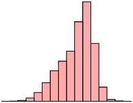
A data set with this frequency polygon:
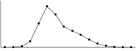
A data set with this distribution:
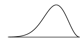
The following data set:
\(\text{105}\) ; \(\text{44}\) ; \(\text{94}\) ; \(\text{149}\) ; \(\text{83}\) ; \(\text{178}\) ; \(-\text{4}\) ; \(\text{112}\) ; \(\text{50}\) ; \(\text{188}\)
The statistics of the data set are
For the following data sets:
\(\text{40}\) ; \(\text{45}\) ; \(\text{12}\) ; \(\text{6}\) ; \(\text{9}\) ; \(\text{16}\) ; \(\text{11}\) ; \(\text{7}\) ; \(\text{35}\) ; \(\text{7}\) ; \(\text{31}\) ; \(\text{3}\)
The mean is \(\bar{x} = \frac{222}{12}=\text{18,5}\).
To determine the five number summary, we order the data:
\[3\ ;\ 6\ ;\ 7\ ;\ 7\ ;\ 9\ ;\ 11\ ;\ 12\ ;\ 16\ ;\ 31\ ;\ 35\ ;\ 40\ ;\ 45\]We use the diagram below (or the formulae) to find at, or between, which values the quartiles lie.

The minimum is 3 and the maximum is 45.
For the first quartile, the position is between the third and fourth values. Since both these values are equal to \(\text{7}\), the first quartile is \(\text{7}\).
For the median (second quartile), the position is halfway between the sixth and seventh values. The sixth value is \(\text{11}\) and the seventh value is \(\text{12}\), which means that the median is \(\frac{11+12}{2}=\text{11,5}\).
For the third quartile, the position is between the ninth and tenth values. Therefore the third quartile is \(\frac{31+35}{2}=33\).
Therefore, the five number summary is (3; 7; \(\text{11,5}\); 33; 45)

Mean \(>\) median, therefore the data is skewed right.
\(\text{65}\) ; \(\text{100}\) ; \(\text{99}\) ; \(\text{21}\) ; \(\text{8}\) ; \(\text{27}\) ; \(\text{21}\) ; \(\text{31}\) ; \(\text{33}\) ; \(\text{31}\) ; \(\text{38}\) ; \(\text{16}\)
The mean is \(\bar{x} = \frac{490}{12}=\text{40,83}\).
To determine the five number summary, we order the data:
\[8\ ;\ 16\ ;\ 21\ ;\ 21\ ;\ 27\ ;\ 31\ ;\ 31\ ;\ 33\ ;\ 38\ ;\ 65\ ;\ 99\ ;\ 100\]We use the formulae (or a diagram) to find at, or between, which values the quartiles lie.
\begin{align*} \text{Location of } Q_{1} & = \frac{1}{4}(n-1)+1 = \frac{1}{4}(12-1)+1 = \text{3,75}\\ \text{Location of } Q_{2} & = \frac{1}{2}(n-1)+1 = \frac{1}{2}(12-1)+1 = \text{6,5}\\ \text{Location of } Q_{3} & = \frac{3}{4}(n-1)+1 = \frac{3}{4}(12-1)+1 = \text{9,25} \end{align*}The minimum is 8 and the maximum is 100.
For the first quartile, the position is between the third and fourth values. Since both these values are equal to \(\text{21}\), the first quartile is \(\text{21}\).
For the median (second quartile), the position is halfway between the sixth and seventh values. The sixth value and seventh value are \(\text{31}\), which means that the median is \(\text{31}\).
For the third quartile, the position is between the ninth and tenth values. Therefore the third quartile is \(\frac{38+65}{2}=\text{51,5}\).
Therefore, the five number summary is (8; 21; \(\text{31}\); \(\text{51,5}\); 100)

Mean \(>\) median, therefore the data is skewed right.
\(\text{65}\) ; \(\text{57}\) ; \(\text{77}\) ; \(\text{92}\) ; \(\text{77}\) ; \(\text{58}\) ; \(\text{90}\) ; \(\text{46}\) ; \(\text{11}\) ; \(\text{81}\)
The mean is \(\bar{x} = \frac{654}{10}=\text{65,4}\).
To determine the five number summary, we order the data:
\[11\ ;\ 46\ ;\ 57\ ;\ 58\ ;\ 65\ ;\ 77\ ;\ 77\ ;\ 81\ ;\ 90\ ;\ 92\]We use the formulae (or a diagram) to find at, or between, which values the quartiles lie.
\begin{align*} \text{Location of } Q_{1} & = \frac{1}{4}(n-1)+1 = \frac{1}{4}(10-1)+1 = \text{3,25}\\ \text{Location of } Q_{2} & = \frac{1}{2}(n-1)+1 = \frac{1}{2}(10-1)+1 = \text{5,5}\\ \text{Location of } Q_{3} & = \frac{3}{4}(n-1)+1 = \frac{3}{4}(10-1)+1 = \text{7,75} \end{align*}The minimum is 11 and the maximum is 92.
For the first quartile, the position is between the third and fourth values. Since the third is 57 and the fourth is 58, the first quartile is \(\frac{57+58}{2}=\text{57,5}\).
For the median (second quartile), the position is halfway between the fifth and sixth values. The sixth value is 65 and the seventh value is \(\text{77}\), therefore the median is \(\frac{65+77}{2}=\text{71}\).
For the third quartile, the position is between the seventh and eighth values. Therefore the third quartile is \(\frac{77+81}{2}=\text{79}\).
Therefore, the five number summary is (11; \(\text{57,5}\); \(\text{77}\); \(\text{79}\); 92)

Mean \(<\) median, therefore the data is skewed left.
\(\text{1}\) ; \(\text{99}\) ; \(\text{76}\) ; \(\text{76}\) ; \(\text{50}\) ; \(\text{74}\) ; \(\text{83}\) ; \(\text{91}\) ; \(\text{41}\) ; \(\text{17}\) ; \(\text{33}\)
The mean is \(\bar{x} = \frac{641}{11}=\text{58,27}\).
To determine the five number summary, we order the data:
\[1\ ;\ 17\ ;\ 33\ ;\ 41\ ;\ 50\ ;\ 74\ ;\ 76\ ;\ 76\ ;\ 83\ ;\ 91\ ;\ 99\]We use the formulae (or a diagram) to find at, or between, which values the quartiles lie.
\begin{align*} \text{Location of } Q_{1} & = \frac{1}{4}(n-1)+1 = \frac{1}{4}(11-1)+1 = \text{3,5}\\ \text{Location of } Q_{2} & = \frac{1}{2}(n-1)+1 = \frac{1}{2}(11-1)+1 = \text{6}\\ \text{Location of } Q_{3} & = \frac{3}{4}(n-1)+1 = \frac{3}{4}(11-1)+1 = \text{8,5} \end{align*}The minimum is 1 and the maximum is 99.
For the first quartile, the position is between the third and fourth values. The third value is 33 and the fourth value is 41, therefore the first quartile is \(\frac{33+41}{2}=\text{37}\).
The second quartile (median) is at the sixth position. The sixth value is \(\text{74}\).
For the third quartile, the position is between the eighth and ninth values. Therefore the third quartile is \(\frac{76+83}{2}=\text{79,5}\).
Therefore, the five number summary is (1; 37; \(\text{74}\); \(\text{79,5}\); 99)

Mean \(<\) median, therefore the data is skewed left.
\(\text{0,5}\); \(-\text{0,9}\) ; \(-\text{1,8}\) ; \(\text{3}\) ; \(-\text{0,2}\) ; \(-\text{5,2}\) ; \(-\text{1,8}\) ; \(\text{0,1}\) ; \(-\text{1,7}\) ; \(-\text{2}\) ; \(\text{2,2}\) ; \(\text{0,5}\); \(-\text{0,5}\)
The mean is \(\bar{x} = \frac{-\text{7,8}}{13}=-\text{0,6}\).
To determine the five number summary, we order the data:
\[-\text{5,2};-\text{2};-\text{1,8};-\text{1,8};-\text{1,7};-\text{0,9};-\text{0,5};-\text{0,2}\ ;\ \text{0,1}\ ;\ \text{0,5}\ ;\ \text{0,5}\ ;\ \text{2,2}\ ;\ \text{3}\]We use the formulae (or a diagram) to find at, or between, which values the quartiles lie.
\begin{align*} \text{Location of } Q_{1} & = \frac{1}{4}(n-1)+1 = \frac{1}{4}(13-1)+1 = \text{4}\\ \text{Location of } Q_{2} & = \frac{1}{2}(n-1)+1 = \frac{1}{2}(13-1)+1 = \text{7}\\ \text{Location of } Q_{3} & = \frac{3}{4}(n-1)+1 = \frac{3}{4}(13-1)+1 = \text{10} \end{align*}The minimum is \(-\text{5,2}\) and the maximum is 3.
The first quartile is at the fourth position. Therefore, the first quartile is \(-\text{1,8}\).
The median (second quartile) is at the seventh position. The seventh value is \(-\text{0,5}\).
The third quartile is at the tenth position. Therefore the third quartile is \(\text{0,5}\).
Therefore, the five number summary is (\(-\text{5,2}\); \(-\text{1,8}\); \(-\text{0,5}\); \(\text{0,5}\); 3)

Mean \(\approx\) median, therefore the data is symmetric.
\(\text{86}\) ; \(\text{64}\) ; \(\text{25}\) ; \(\text{71}\) ; \(\text{54}\) ; \(\text{44}\) ; \(\text{97}\) ; \(\text{31}\) ; \(\text{78}\) ; \(\text{46}\) ; \(\text{60}\) ; \(\text{86}\)
The mean is \(\bar{x} = \frac{742}{12}=\text{61,83}\).
To determine the five number summary, we order the data:
\[25\ ;\ 31\ ;\ 44\ ;\ 46\ ;\ 54\ ;\ 60\ ;\ 64\ ;\ 71\ ;\ 78\ ;\ 86\ ;\ 86\ ;\ 97\]We use the formulae (or a diagram) to find at, or between, which values the quartiles lie.
\begin{align*} \text{Location of } Q_{1} & = \frac{1}{4}(n-1)+1 = \frac{1}{4}(12-1)+1 = \text{3,75}\\ \text{Location of } Q_{2} & = \frac{1}{2}(n-1)+1 = \frac{1}{2}(12-1)+1 = \text{6,5}\\ \text{Location of } Q_{3} & = \frac{3}{4}(n-1)+1 = \frac{3}{4}(12-1)+1 = \text{9,25} \end{align*}The minimum is 25 and the maximum is 97.
For the first quartile, the position is between the third and fourth values. The third value is 44 and the fourth value is \(\text{46}\), which means that the first quartile is \(\frac{44+46}{2}=\text{45}\).
For the median (second quartile), the position is halfway between the sixth and seventh values. The sixth value is 60 and the seventh value is \(\text{64}\), which means that the median is \(\frac{60+64}{2}=\text{62}\).
For the third quartile, the position is between the ninth and tenth values. Therefore the third quartile is \(\frac{78+86}{2}=\text{82}\).
Therefore, the five number summary is (25; 45; \(\text{62}\); \(\text{82}\); 97)

Mean \(\approx\) median, therefore the data is symmetric.
For the following data sets:
\(\{\text{9,1}; \text{0,2}; \text{2,8}; \text{2,0}; \text{10,0}; \text{5,8}; \text{9,3}; \text{8,0}\}\)
The formula for the mean is
\begin{align*} \bar{x} &= \frac{\sum\limits_{i=1}^n x_i}{n} \\ \therefore \bar{x} &= \frac{\text{47,2}}{8} \\ &= \text{5,90} \end{align*}The formula for the variance is \[\sigma^2 = \frac{\sum_{i=1}^n \left(x_i - \overline{x}\right)^2}{n}\]
We first subtract the mean from each data point and then square the result.
| \(x_i\) | \(\text{9,1}\) | \(\text{0,2}\) | \(\text{2,8}\) | \(\text{2,0}\) | \(\text{10,0}\) | \(\text{5,8}\) | \(\text{9,3}\) | \(\text{8,0}\) |
| \(x_i - \overline{x}\) | \(\text{3,2}\) | \(-\text{5,7}\) | \(-\text{3,1}\) | \(-\text{3,9}\) | \(\text{4,1}\) | \(-\text{0,1}\) | \(\text{3,4}\) | \(\text{2,1}\) |
| \((x_i - \overline{x})^2\) | \(\text{10,24}\) | \(\text{32,49}\) | \(\text{9,61}\) | \(\text{15,21}\) | \(\text{16,81}\) | \(\text{0,01}\) | \(\text{11,56}\) | \(\text{4,41}\) |
The variance is the sum of the last row in this table divided by \(\text{8}\), so \(\sigma^2 = \frac{\text{47,2}}{8}=\text{12,54}\). The standard deviation is the square root of the variance, therefore \(\sigma=\sqrt{12.54}=\pm \text{3,54}\).
The interval containing all values that are one standard deviation from the mean is \(\left[\text{5,90}-\text{3,54} ; \text{5,90}+\text{3,54}\right] = \left[\text{9,44} ; \text{2,36}\right]\). We are asked how many values are within than one standard deviation from the mean, meaning inside the interval. There are \(\text{5}\) values from the data set within the interval, which is \(\frac{5}{8} \times 100=\text{63}\%\) of the data points.
\{9; 5; 1; 3; 3; 5; 7; 4; 10; 8\}
The formula for the mean is
\begin{align*} \bar{x} &= \frac{\sum\limits_{i=1}^n x_i}{n} \\ \therefore \bar{x} &= \frac{55}{10} \\ &= \text{5,5} \end{align*}The formula for the variance is \[\sigma^2 = \frac{\sum_{i=1}^n \left(x_i - \overline{x}\right)^2}{n}\]
We first subtract the mean from each data point and then square the result.
| \(x_i\) | \(\text{9}\) | \(\text{5}\) | \(\text{1}\) | \(\text{3}\) | \(\text{3}\) | \(\text{5}\) | \(\text{7}\) | \(\text{4}\) | \(\text{10}\) | \(\text{8}\) |
| \(x_i - \overline{x}\) | \(\text{3,5}\) | \(-\text{0,5}\) | \(-\text{4,5}\) | \(-\text{2,5}\) | \(-\text{2,5}\) | \(-\text{0,5}\) | \(\text{1,5}\) | \(-\text{1,5}\) | \(\text{4,5}\) | \(\text{2,5}\) |
| \((x_i - \overline{x})^2\) | \(\text{12,25}\) | \(\text{0,25}\) | \(\text{20,25}\) | \(\text{6,25}\) | \(\text{6,25}\) | \(\text{0,25}\) | \(\text{2,25}\) | \(\text{2,25}\) | \(\text{20,25}\) | \(\text{6,25}\) |
The variance is the sum of the last row in this table divided by \(\text{10}\), so \(\sigma^2 = \frac{\text{76,5}}{\text{10}} = \text{7,65}\). The standard deviation is the square root of the variance, therefore \(\sigma=\sqrt{\text{7,65}}=\pm \text{2,77}\).
The interval containing all values that are one standard deviation from the mean is \(\left[\text{5,5}-\text{2,77} ; \text{5,5}+\text{2,77}\right] = \left[\text{2,73} ; \text{8,27}\right]\). We are asked how many values are within than one standard deviation from the mean, meaning inside the interval. There are \(\text{7}\) values from the data set within the interval, which is \(\frac{7}{10} \times 100=\text{70}\%\) of the data points.
\{81; 22; 63; 12; 100; 28; 54; 26; 50; 44; 4; 32\}
The formula for the mean is
\begin{align*} \bar{x} &= \frac{\sum\limits_{i=1}^n x_i}{n} \\ \therefore \bar{x} &= \frac{516}{12} \\ &= \text{43} \end{align*}The formula for the variance is \[\sigma^2 = \frac{\sum_{i=1}^n \left(x_i - \overline{x}\right)^2}{n}\]
We first subtract the mean from each data point and then square the result.
| \(x_i\) | \(\text{81}\) | \(\text{22}\) | \(\text{63}\) | \(\text{12}\) | \(\text{100}\) | \(\text{28}\) | \(\text{54}\) | \(\text{26}\) | \(\text{50}\) | \(\text{44}\) | \(\text{4}\) | \(\text{32}\) |
| \(x_i - \overline{x}\) | \(\text{38}\) | \(-\text{21}\) | \(\text{20}\) | \(-\text{31}\) | \(\text{57}\) | \(-\text{15}\) | \(\text{11}\) | \(-\text{17}\) | \(\text{7}\) | \(\text{1}\) | \(-\text{39}\) | \(-\text{11}\) |
| \((x_i - \overline{x})^2\) | \(\text{1 444}\) | \(\text{441}\) | \(\text{400}\) | \(\text{961}\) | \(\text{3 249}\) | \(\text{225}\) | \(\text{121}\) | \(\text{289}\) | \(\text{49}\) | \(\text{1}\) | \(\text{1 521}\) | \(\text{121}\) |
The variance is the sum of the last row in this table divided by \(\text{12}\), so \(\sigma^2 = \frac{\text{8 822}}{12}=\text{735,17}\). The standard deviation is the square root of the variance, therefore \(\sigma=\sqrt{735.17}=\pm \text{27,11}\).
The interval containing all values that are one standard deviation from the mean is \(\left[\text{43}-\text{27,11} ; \text{43}+\text{27,11}\right] = \left[\text{15,89} ; \text{70,11}\right]\). We are asked how many values are within than one standard deviation from the mean, meaning inside the interval. There are \(\text{8}\) values from the data set within the interval, which is \(\frac{8}{12} \times 100=\text{67}\%\) of the data points.
Use a calculator to determine the
\(\text{8}\) ; \(\text{3}\) ; \(\text{10}\) ; \(\text{7}\) ; \(\text{7}\) ; \(\text{1}\) ; \(\text{3}\) ; \(\text{1}\) ; \(\text{3}\) ; \(\text{7}\)
\(\text{4}\) ; \(\text{4}\) ; \(\text{13}\) ; \(\text{9}\) ; \(\text{7}\) ; \(\text{7}\) ; \(\text{2}\) ; \(\text{5}\) ; \(\text{15}\) ; \(\text{4}\) ; \(\text{22}\) ; \(\text{11}\)
\(\text{4,38}\) ; \(\text{3,83}\) ; \(\text{4,99}\) ; \(\text{4,05}\) ; \(\text{2,88}\) ; \(\text{4,83}\) ; \(\text{0,88}\) ; \(\text{5,33}\) ; \(\text{3,49}\) ; \(\text{4,10}\)
\(\text{4,76}\) ; \(-\text{4,96}\) ; \(-\text{6,35}\) ; \(-\text{3,57}\) ; \(\text{0,59}\) ; \(-\text{2,18}\) ; \(-\text{4,96}\) ; \(-\text{3,57}\) ; \(-\text{2,18}\) ; \(\text{1,98}\)
\(\text{7}\) ; \(\text{53}\) ; \(\text{29}\) ; \(\text{42}\) ; \(\text{12}\) ; \(\text{111}\) ; \(\text{122}\) ; \(\text{79}\) ; \(\text{83}\) ; \(\text{5}\) ; \(\text{69}\) ; \(\text{45}\) ; \(\text{23}\) ; \(\text{77}\)
Xolani surveyed the price of a loaf of white bread at two different supermarkets. The data, in rands, are given below.
| Supermarket A | \(\text{3,96}\) | \(\text{3,76}\) | \(\text{4,00}\) | \(\text{3,91}\) | \(\text{3,69}\) | \(\text{3,72}\) |
| Supermarket B | \(\text{3,97}\) | \(\text{3,81}\) | \(\text{3,52}\) | \(\text{4,08}\) | \(\text{3,88}\) | \(\text{3,68}\) |
Supermarket A: \(\text{3,84}\). Supermarket B: \(\text{3,82}\). Supermarket B has the lower mean.
Standard deviation: \[\sigma = \sqrt{\frac{\sum\limits_{i=1}^n \left(x_i - \bar{x}\right)^2}{n}}\]
For Supermarket A: \begin{align*} \sigma &= \sqrt{\frac{\sum\limits_{i=1}^n \left(x_i - \text{3,84}\right)^2}{\text{6}}} \\ &= \sqrt{\frac{\text{0,0882}}{\text{6}}} \\ &= \sqrt{\text{0,0147}} \\ &\approx \pm \text{0,121} \end{align*}
For Supermarket B: \begin{align*} \sigma &= \sqrt{\frac{\sum\limits_{i=1}^n \left(x_i - \text{3,82}\right)^2}{6}} \\ &= \sqrt{\frac{\text{0,20}\dot{3}}{\text{6}}} \\ &= \sqrt{\text{0,033}\dot{8}} \\ &\approx \pm\text{0,184} \end{align*}
The standard deviation of Supermarket A's prices is lower than that of Supermarket B's. That means that Supermarket A has more consistent (less variable) prices than Supermarket B.
The times for the \(\text{8}\) athletes who swam the \(\text{100}\) \(\text{m}\) freestyle final at the 2012 London Olympic Games are shown below. All times are in seconds.
\(\text{47,52}\) ; \(\text{47,53}\) ; \(\text{47,80}\) ; \(\text{47,84}\) ; \(\text{47,88}\) ; \(\text{47,92}\) ; \(\text{48,04}\) ; \(\text{48,44}\)
The mean is \(\text{47,87}\) and the standard deviation is \(\text{0,56}\). Therefore the interval containing all values that are one standard deviation from the mean is \(\left[\text{47,87}-\text{0,27} ; \text{47,87}+\text{0,27}\right] = \left[\text{47,60} ; \text{48,15}\right]\). We are asked how many values are further than one standard deviation from the mean, meaning outside the interval. There are \(\text{3}\) values from the data set outside the interval.
The following data set has a mean of \(\text{14,7}\) and a variance of \(\text{10,01}\).
\[\text{18}\ ;\ \text{11}\ ;\ \text{12}\ ;\ a\ ;\ \text{16}\ ;\ \text{11}\ ;\ \text{19}\ ;\ \text{14}\ ;\ b\ ;\ \text{13}\]Calculate the values of \(a\) and \(b\).
From the formula of the mean we have \begin{align*} \text{14,7} &= \frac{\text{114} + a + b}{10} \\ \therefore a + b &= \text{147} - \text{114} \\ \therefore a &= 33-b \end{align*}
From the formula of the variance we have \begin{align*} \sigma^2 &= \frac{\sum_{i=1}^n (x_i-\overline{x})^2}{n} \\ \therefore \text{10,01} &= \frac{\text{69,12} + (a-\text{14,7})^2 + (b-\text{14,7})^2}{10} \end{align*}
Substitute \(a = 33-b\) into this equation to get \begin{align*} \text{10,01} &= \frac{\text{69,12} + (\text{18,3}-b)^2 + (b-\text{14,7})^2}{10} \\ \therefore \text{100,1} &= 2b^2 - \text{66}b + \text{620,1} \\ \therefore 0 &= b^2 - \text{33}b + \text{260} \\ &= (b-13)(b-20) \end{align*} Therefore \(b = 13\) or \(b = 20\).
Since \(a = 33-b\) we have \(a = 20\) or \(a = 13\). So, the two unknown values in the data set are \(\text{13}\) and \(\text{20}\).
We do not know which of these is \(a\) and which is \(b\) since the mean and variance tell us nothing about the order of the data.
The height of each learner in a class was measured and it was found that the mean height of the class was \(\text{1,6}\) \(\text{m}\). At the time, three learners were absent. However, when the heights of the learners who were absent were included in the data for the class, the mean height did not change.
If the heights of two of the learners who were absent are \(\text{1,45}\) \(\text{m}\) and \(\text{1,63}\) \(\text{m}\), calculate the height of the third learner who was absent. [NSC Paper 3 Feb-March 2013]
Let the number of learners who were first measured be \(x\).
The total measure of all heights is \(\text{1,6}x\).
Let the height of the last learner be \(y\).
\begin{align*} \frac{\text{1,6}x+\text{1,45}+\text{1,63}+y}{x+3}&=\text{1,6} \\ \text{1,6}x + \text{3,08} + y&= \text{1,6}x + \text{4,8} \\ y&=\text{1,72} \end{align*}There are 184 students taking Mathematics in a first-year university class. The marks, out of 100, in the half-yearly examination are normally distributed with a mean of 72 and a standard deviation of 9. [NSC Paper 3 Feb-March 2013]
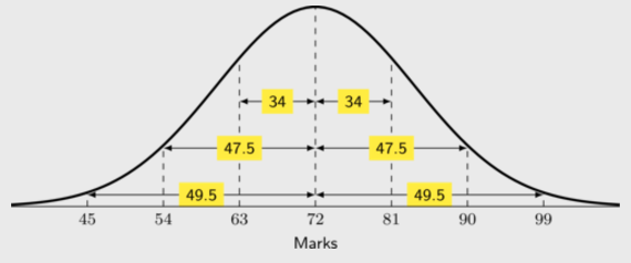
\(90=72 +2(9)\)
Therefore 90 lies at 2 standard deviations to the right of the mean.
Hence, \(\text{47,5}\%\) of students scored between 72 and 90 marks.
|
Previous
End of chapter exercises
|
Table of Contents |
Next
9.2 Curve fitting
|