\(140-12=128\)
128 is 1 standard deviation to the left of the mean, therefore the percentage of teenagers who sent less than 128 messages is:
\(\text{50}\% - \text{34}\% = \text{16}\%\)
|
Previous
9.4 Summary
|
Next
10.1 Revision
|
The number of SMS messages sent by a group of teenagers was recorded over a period of a week. The data was found to be normally distributed with a mean of 140 messages and a standard deviation of 12 messages. [NSC Paper 3 Feb-March 2012]
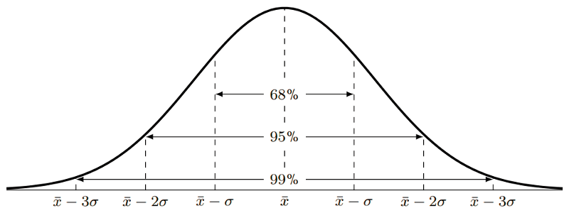
Answer the following questions with reference to the information provided in the graph:
\(140-12=128\)
128 is 1 standard deviation to the left of the mean, therefore the percentage of teenagers who sent less than 128 messages is:
\(\text{50}\% - \text{34}\% = \text{16}\%\)
116 minutes is 2 standard deviations from the mean, therefore \(\text{47,5}\%\)
152 minutes is 1 standard deviation from the mean, therefore \(\text{34}\%\)
Percentage of the teenagers who sent between 116 and 152 messages \(= \text{47,5}\% + \text{34}\% = \text{81,5}\%\)
A company produces sweets using a machine which runs for a few hours per day. The number of hours running the machine and the number of sweets produced are recorded.
| Machine hours | Sweets produced |
| \(\text{3,80}\) | \(\text{275}\) |
| \(\text{4,23}\) | \(\text{287}\) |
| \(\text{4,37}\) | \(\text{291}\) |
| \(\text{4,10}\) | \(\text{281}\) |
| \(\text{4,17}\) | \(\text{286}\) |
Find the linear regression equation for the data, and estimate the machine hours needed to make \(\text{300}\) sweets.
Using a calculator, the equation is:
\[\hat{y} = \text{165,70} + \text{28,62}x\]Therefore, the estimated number of machine hours needed to make 300 sweets is:
\begin{align*} 300 &= \text{165,70} + \text{28,62}x \\ \therefore x &= \frac{300-\text{165,7}}{\text{28,62}} = \text{4,69} \text{ machine hours} \end{align*}The profits of a new shop are recorded over the first 6 months. The owner wants to predict his future sales. The profits by month so far have been \(\text{R}\,\text{90 000}\); \(\text{R}\,\text{93 000}\); \(\text{R}\,\text{99 500}\); \(\text{R}\,\text{102 000}\); \(\text{R}\,\text{101 300}\); \(\text{R}\,\text{109 000}\).
Calculate the linear regression function for the data, using profit as your \(y\)-variable. Round \(a\) and \(b\) to two decimal places.
Give an estimate of the profits for the next two months.
The owner wants a profit of \(\text{R}\,\text{130 000}\). Estimate how many months this will take.
It will take 13 months to reach a profit of \(\text{R}\,\text{130 000}\).
A fast food company produces hamburgers. The number of hamburgers made and the costs are recorded over a week.
| Hamburgers made | Costs |
| \(\text{495}\) | \(\text{R}\,\text{2 382}\) |
| \(\text{550}\) | \(\text{R}\,\text{2 442}\) |
| \(\text{515}\) | \(\text{R}\,\text{2 484}\) |
| \(\text{500}\) | \(\text{R}\,\text{2 400}\) |
| \(\text{480}\) | \(\text{R}\,\text{2 370}\) |
| \(\text{530}\) | \(\text{R}\,\text{2 448}\) |
| \(\text{585}\) | \(\text{R}\,\text{2 805}\) |
Find the linear regression function that best fits the data. Use hamburgers made as your \(x\)-variable and round \(a\) and \(b\) to two decimal places.
Calculate the value of the correlation coefficient, correct to two decimal places, and comment on the strength and direction of the correlation.
There is a strong, positive, linear correlation.
If the total cost in a day is \(\text{R}\,\text{2 500}\), estimate the number of hamburgers produced. Round your answer down to the nearest whole number.
Therefore 528 burgers are produced.
What is the cost of \(\text{490}\) hamburgers?
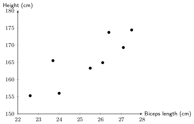
A collection of data related to an investigation into biceps length and height of students was recorded in the table below. Answer the questions to follow.
| Length of right biceps (cm) | Height (cm) |
| \(\text{25,5}\) | \(\text{163,3}\) |
| \(\text{26,1}\) | \(\text{164,9}\) |
| \(\text{23,7}\) | \(\text{165,5}\) |
| \(\text{26,4}\) | \(\text{173,7}\) |
| \(\text{27,5}\) | \(\text{174,4}\) |
| \(\text{24}\) | \(\text{156}\) |
| \(\text{22,6}\) | \(\text{155,3}\) |
| \(\text{27,1}\) | \(\text{169,3}\) |
Draw a scatter plot of the data set.
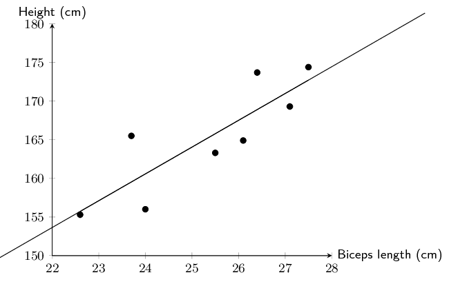
Calculate equation of the line of regression.
Draw the regression line onto the graph.
Calculate the correlation coefficient \(r\)
What conclusion can you reach, regarding the relationship between the length of the right biceps and height of the students in the data set?
The length of the right biceps and the height of the students have a strong, positive linear relationship.
A class wrote two tests, and the marks for each were recorded in the table below. Full marks in the first test was \(\text{50}\), and the second test was out of \(\text{30}\).
| Learner | Test 1 | Test 2 |
| (Full marks: \(\text{50}\)) | (Full marks: \(\text{30}\)) | |
| \(\text{1}\) | \(\text{42}\) | \(\text{25}\) |
| \(\text{2}\) | \(\text{32}\) | \(\text{19}\) |
| \(\text{3}\) | \(\text{31}\) | \(\text{20}\) |
| \(\text{4}\) | \(\text{42}\) | \(\text{26}\) |
| \(\text{5}\) | \(\text{35}\) | \(\text{23}\) |
| \(\text{6}\) | \(\text{23}\) | \(\text{14}\) |
| \(\text{7}\) | \(\text{43}\) | \(\text{24}\) |
| \(\text{8}\) | \(\text{23}\) | \(\text{12}\) |
| \(\text{9}\) | \(\text{24}\) | \(\text{14}\) |
| \(\text{10}\) | \(\text{15}\) | \(\text{10}\) |
| \(\text{11}\) | \(\text{19}\) | \(\text{11}\) |
| \(\text{12}\) | \(\text{13}\) | \(\text{10}\) |
| \(\text{13}\) | \(\text{36}\) | \(\text{22}\) |
| \(\text{14}\) | \(\text{29}\) | \(\text{17}\) |
| \(\text{15}\) | \(\text{29}\) | \(\text{17}\) |
| \(\text{16}\) | \(\text{25}\) | \(\text{16}\) |
| \(\text{17}\) | \(\text{29}\) | \(\text{18}\) |
| \(\text{18}\) | \(\text{17}\) | |
| \(\text{19}\) | \(\text{30}\) | \(\text{19}\) |
| \(\text{20}\) | \(\text{28}\) | \(\text{17}\) |
Is there a strong correlation between the marks for the first and second test? Show why or why not.
Using a calculator, \(r=\text{0,98}\) which is a very strong, positive, linear correlation between the marks of the first and the second test.
One of the learners (in Row 18) did not write the second test. Given her mark for the first test, calculate an expected mark for the second test. Round the mark up to the nearest whole number.
Using a calculator, the least squares regression line equation is:
\[\hat{y} = \text{1,08} + \text{0,57}x\]Therefore, the expected mark for the second test for the learner in Row 18 is:
\[y = \text{1,08} + \text{0,57}(17) = \text{10,77}\]Therefore the expected mark for the learner in row 18 for the second test is 11 out of 30.
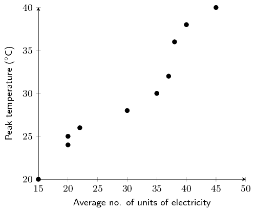
Lindiwe works for Eskom, the South African power distributor. She knows that on hot days more electricity than average is used to cool houses. In order to accurately predict how much more electricity needs to be produced, she wants to determine the precise nature of the relationship between temperature and electricity usage.
The data below shows the peak temperature in degrees Celsius on ten consecutive days during summer and the average number of units of electricity used by a number of households. Examine her data and answer the questions that follow.
| Peak temp. (\(y\)) | 32 | 40 | 30 | 28 | 25 | 38 | 36 | 20 | 24 | 26 |
| Average no. of units (\(x\)) | 37 | 45 | 35 | 30 | 20 | 40 | 38 | 15 | 20 | 22 |
| Average no. of units (\(x\)) | Peak temp. (\(y\)) | \(xy\) | \(x^{2}\) |
| 37 | 32 | \(\text{1 184}\) | \(\text{1 369}\) |
| 45 | 40 | \(\text{1 800}\) | \(\text{2 025}\) |
| 35 | 30 | \(\text{1 050}\) | 1225 |
| 30 | 28 | 840 | 900 |
| 20 | 25 | 500 | 400 |
| 40 | 38 | \(\text{1 520}\) | \(\text{1 600}\) |
| 38 | 36 | \(\text{1 368}\) | \(\text{1 444}\) |
| 15 | 20 | \(\text{300}\) | \(\text{225}\) |
| 20 | 24 | \(\text{480}\) | \(\text{400}\) |
| 22 | 26 | \(\text{572}\) | \(\text{484}\) |
| \(\sum = 302\) | \(\sum = 299\) | \(\sum = \text{9 614}\) | \(\sum = \text{10 072}\) |
We have already calculated the value of \(b\) by hand in the question above, so we are left to determine \(\sigma_{x}\) and \(\sigma_{y}\).
| Average no. of units (\(x\)) | Peak temp. (\(y\)) | \((x-\bar{x})^{2}\) | \((y-\bar{y})^{2}\) |
| 32 | 37 | \(\text{46,24}\) | \(\text{4,41}\) |
| 40 | 45 | \(\text{219,04}\) | \(\text{102,01}\) |
| 30 | 35 | \(\text{0,01}\) | \(\text{23,04}\) |
| 28 | 30 | \(\text{0,04}\) | \(\text{3,61}\) |
| 25 | 20 | \(\text{104,04}\) | \(\text{24,01}\) |
| 38 | 40 | \(\text{96,04}\) | \(\text{65,61}\) |
| 36 | 38 | \(\text{60,84}\) | \(\text{37,21}\) |
| 20 | 15 | \(\text{231,04}\) | \(\text{98,01}\) |
| 24 | 20 | \(\text{104,04}\) | \(\text{34,81}\) |
| 26 | 22 | \(\text{67,24}\) | \(\text{15,21}\) |
| \(\sum=299\) | \(\sum=\text{302}\) | \(\sum=\text{951,6}\) | \(\sum=\text{384,9}\) |
There is a very strong, positive, linear correlation between peak temperature and the average number of electricity units a household uses.
The value we were asked to predict is outside the range of the available data. This is known as extrapolation.
Lindiwe suspected that the relationship between temperature and electricity consumption was not linear for all temperatures. She then decided to collect data for peak temperatures down to \(\text{0}\)\(\text{°C}\). Examine the graph of her data below and identify which type of function would best fit the data and describe the nature of the relationship between temperature and electricity for the newly available data.
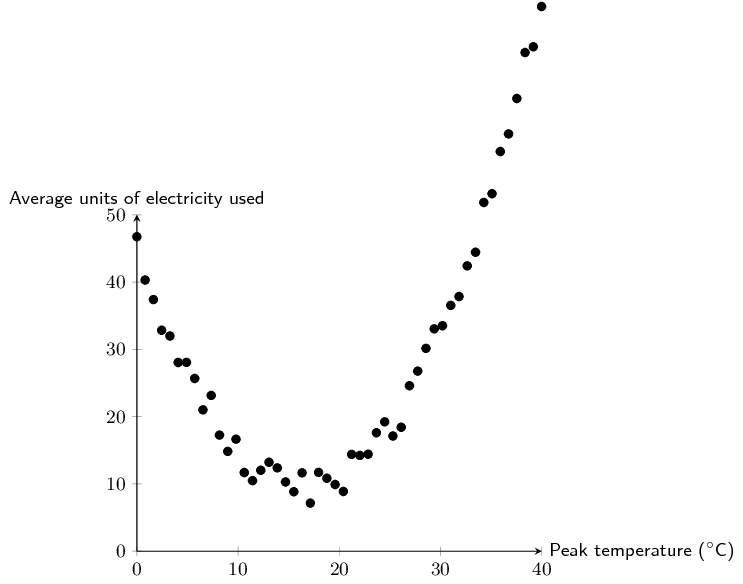
A quadratic function would best fit the data. At about \(\text{18}\)\(\text{°C}\) average household electricity usage is at its minimum. As the peak temperature gets colder or warmer than this point, electrcity usage increases.
Lindiwe is asked by her superiors to determine which day is best to perform maintenance on one of their power plants. She determined that the equation \(y=\text{0,13}x^2 - \text{4,3}x + 45\) best fit her data. Use her equation to estimate the peak temperature and average no. of units used on the day when the least amount of electricity generation is required.
This question requires us to find the minimum value of the quadratic equation. There are a number of ways to do this, two are shown below:
The first method is using the formula \(x = \frac{-b}{2a}\):
Another method is using differentiation:
Therefore the peak temperature when electricity demand is at its lowest is \(\text{16,54}\)\(\text{°C}\) and the respective average household electricity usage is \(\text{9,44}\) \(\text{units}\).
Below is a list of data concerning 12 countries and their respective carbon dioxide \((\text{CO}_{2})\) emission levels per person per annum (measured in tonnes) and the gross domestic product (GDP is a measure of products produced and services delivered within a country in a year) per person (in US dollars). Data sourced from the World Bank and the US Department of Energy's Carbon Dioxide Information Analysis Center.
| \(\text{CO}_{2}\) emmissions per capita (x) | GDP per capita (y) | |
| South Africa | \(\text{8,8}\) | \(\text{11 440}\) |
| Thailand | \(\text{4,1}\) | \(\text{9 815}\) |
| Italy | \(\text{7,5}\) | \(\text{32 512}\) |
| Australia | \(\text{18,3}\) | \(\text{44 462}\) |
| China | \(\text{5,3}\) | \(\text{9 233}\) |
| India | \(\text{1,4}\) | \(\text{3 876}\) |
| Canada | \(\text{15,3}\) | \(\text{42 693}\) |
| United Kingdom | \(\text{8,5}\) | \(\text{35 819}\) |
| United States | \(\text{17,2}\) | \(\text{49 965}\) |
| Saudi Arabia | \(\text{16,1}\) | \(\text{24 571}\) |
| Iran | \(\text{7,3}\) | \(\text{11 395}\) |
| Indonesia | \(\text{1,8}\) | \(\text{4 956}\) |
Draw a scatter plot of the data set.
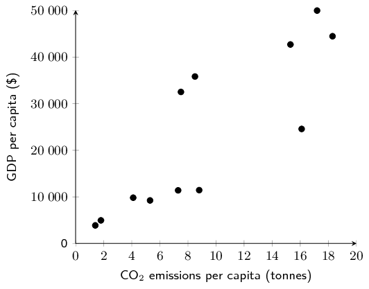
Draw your estimate of the line of best fit on your scatter plot and determine the equation of your line of best fit.
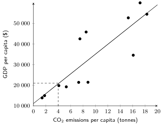
The \(y\)-intercept is approximately 1000. At \(x=4\), \(y\) is approximately \(\text{11 000}\). Therefore, \(m = \frac{\Delta y}{\Delta x} = \frac{11000-1000}{4-0} = \text{2 500}\)
The equation for the line of best fit: \(y = \text{2 500}x + \text{1 000}\)
Use your calculator to determine the equation for the least squares regression line. Round \(a\) and \(b\) to two decimal places in your final answer.
\(a = \text{1 133,996106}\) and \(b = \text{2 393,736978}\), therefore \(\hat{y} = \text{1 134,00} + \text{2 393,74}x\)
Use your calculator to determine the correlation coefficient, \(r\). Round your answer to two decimal places.
What conclusion can you reach regarding the relationship between \(\text{CO}_{2}\) emissions per annum and GDP per capita for the countries in the data set?
There is a strong, positive, linear correlation between \(\text{CO}_{2}\) emissions per annum and GDP per capita for the countries in the data set.
Kenya has a GDP per capita of \(\text{\$}\,\text{1 712}\). Use your equation of the least squares regression line to estimate the annual \(\text{CO}_{2}\) emissions of Kenya correct to two decimal places.
A group of students attended a course in Statistics on Saturdays over a period of 10 months. The number of Saturdays on which a student was absent was recorded against the final mark the student obtained. The information is shown in the table below. [Adapted from NSC Paper 3 Feb-March 2012]
| Number of Saturdays absent | 0 | 1 | 2 | 2 | 3 | 3 | 5 | 6 | 7 |
| Final mark (as \(\%\)) | \(\text{96}\) | \(\text{91}\) | \(\text{78}\) | \(\text{83}\) | \(\text{75}\) | \(\text{62}\) | \(\text{70}\) | \(\text{68}\) | \(\text{56}\) |
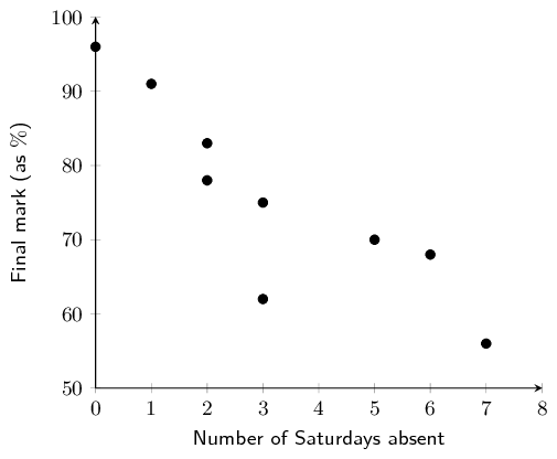
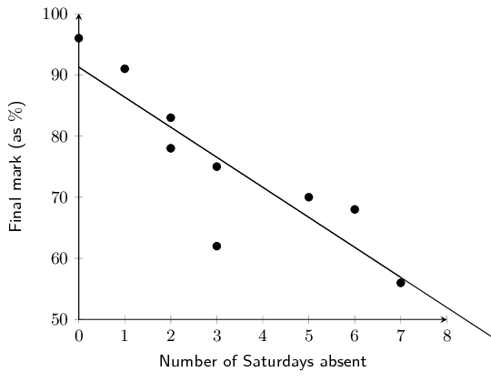
The greater the number of Saturdays absent, the lower the mark.
Grant and Christie are training for a half-marathon together in 8 weeks time. Christie is much fitter than Grant but she has challenged him to beat her time at the race. Grant has begun a rigid training programme to try and improve his time.
Time taken to complete a half marathon was recorded each Sunday. The first recorded Sunday is denoted as week 1. The half-marathon takes place on the eighth Sunday, i.e. week 8. Examine the data set in the table below and answer the questions the follow.
| Week | 1 | 2 | 3 | 4 | 5 | 6 |
| Grant's time (HH:MM) | 02:01 | 01:59 | 01:55 | 01:53 | 01:47 | 01:42 |
| Christie's time (HH:MM) | 01:40 | 01:42 | 01:38 | 01:39 | 01:37 | 01:35 |
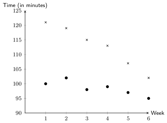
Both data sets show negative, linear trends. The trend in Grant's data appears to be more rapidly decreasing than the trend in Christie's data.
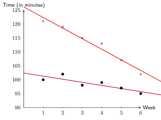
Grant will beat Christie when \(\hat{y}_{\text{Grant}} < \hat{y}_{\text{Christie}}\). To find where the trends intersect, we equate each \(\hat{y}\).
\begin{align*} \text{126,13} -\text{3,8}x &= \text{102,4} - \text{1,11}x \\ -\text{3,8}x + \text{1,11}x&= \text{102,4} - \text{126,13} \\ -\text{2,69}x &= -\text{23,73} \\ x &= \text{8,82} \end{align*}The race takes place in week 8. \(\text{8,82} > 8\), therefore, Grant will be unable to beat Christie's time when the race takes place.
See answer to e). Grant will be able to beat Christie's time in the ninth week.
|
Previous
9.4 Summary
|
Table of Contents |
Next
10.1 Revision
|