9.3 Correlation | Statistics

9.3 Correlation (EMCJS)

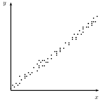
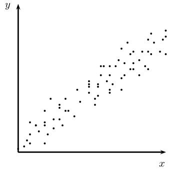
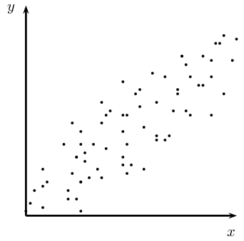
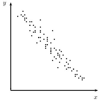
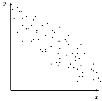
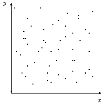
The linear correlation coefficient, \(r\), is a measure which tells us the strength and direction of a relationship between two variables. The correlation coefficient \(r\in \left[-1;1\right]\). When \(r=-1\), there is perfect negative correlation, when \(r=0\), there is no correlation and when \(r=1\) there is perfect positive correlation.


Positive, strong	Positive, fairly strong	Positive, weak
\(r\approx \text{0,9}\)	\(r\approx \text{0,7}\)	\(r\approx \text{0,4}\)


Negative, fairly strong	Negative, weak	No correlation
\(r\approx -\text{0,7}\)	\(r\approx -\text{0,4}\)	\(r=0\)

NB. See the fifth bullet at the beginning of the chapter regarding the formula for the correlation coefficient.

The linear correlation coefficient \(r\) can be calculated using the formula

\(r=b\dfrac{\sigma_{x}}{\sigma_{y}}\)

where \(b\) is the gradient of the least squares regression line,
\(\sigma_{x}\) is the standard deviation of the \(x\)-values and
\(\sigma_{y}\) is the standard deviation of the \(y\)-values.

This is known as the Pearson's product moment correlation coefficient. It is much easier to do on a calculator where you simply follow the procedure for the regression equation, and go on to find \(r\).

In general:

Positive	Strength	Negative
\(r=0\)	no correlation	\(r=0\)
\(0<r<\text{0,25}\)	very weak	\(-\text{0,25}<r<0\)
\(\text{0,25}<r<\text{0,5}\)	weak	\(-\text{0,5}<r<-\text{0,25}\)
\(\text{0,5}<r<\text{0,75}\)	moderate	\(-\text{0,75}<r<-\text{0,5}\)
\(\text{0,75}<r<\text{0,9}\)	strong	\(-\text{0,9}<r<-\text{0,75}\)
\(\text{0,9}<r<1\)	very strong	\(-\text{1}<r<-0.9\)
\(r=1\)	perfect correlation	\(r=-1\)

Correlation does not imply causation! Just because two variables are correlated does not mean that they are causally linked, i.e. if A and B are correlated, that does not mean A causes B, or vice versa. This is a common mistake made by many people, especially journalists looking for their next juicy story.

For example, ice cream sales and shark attacks are correlated. This does not mean that the sale of ice cream is somehow causing more shark attacks. Instead, a simpler explanation is that the warmer it is, the more likely people are to buy ice cream and the more likely people are to go to the beach as well, thus increasing the likelihood of a shark attack.

Video: 29DV

temp text

Worked example 9: The correlation coefficient

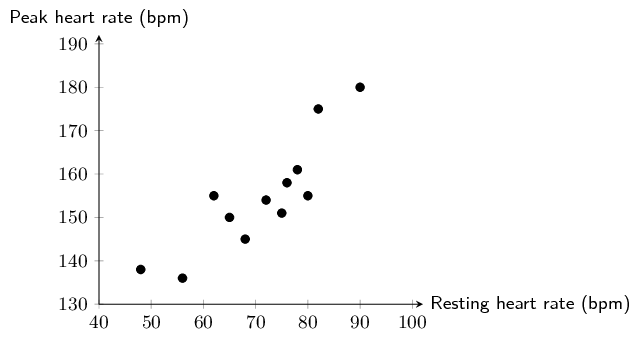
A cardiologist wanted to test the relationship between resting heart rate and the peak heart rate during exercise. Heart rate is measured in beats per minute (bpm). The following set of data was generated from 12 study participants after they had run on a treadmill at \(\text{10}\) \(\text{km/h}\) for 10 minutes.

Resting heart rate	48	56	90	65	75	78	80	72	82	76	68	62
Peak heart rate	138	136	180	150	151	161	155	154	175	158	145	155

Draw a scatter plot of the data. Use resting heart rate as your \(x\)-variable.
Use your calculator to determine the equation of the line of best fit.
Estimate what the heart rate of a person with a resting heart rate of \(\text{70}\) \(\text{bpm}\) will be after exercise.
Without using your calculator, find the correlation coefficient, \(r\). Confirm your answer using your calculator.
What can you conclude regarding the relationship between resting heart rate and the heart rate after exercise?

Draw the scatter plot

Choose a suitable scale for the axes.
Draw the axes.
Plot the points.

Calculate the equation of the line of best fit

As you learnt previously, use your calculator to determine the values for \(a\) and \(b\).

\(a = \text{86,75}\)

\(b = \text{0,96}\)

Therefore, the equation for the line of best fit is \(y = \text{86,75} + \text{0,96}x\)

Calculate the estimated value for \(y\)

If \(x = 70\), using our equation, the estimated value for \(y\) is: \[y= \text{86,75} + \text{0,96} \times 70 = \text{153,95}\]

Calculate the correlation co-efficient

The formula for \(r\) is:

\[r=b\dfrac{\sigma_{x}}{\sigma_{y}}\]

We already know the value of \(b\) and you know how to calculate \(b\) by hand from worked example 5, so we are just left to determine the value for \(\sigma_{x}\) and \(\sigma_{y}\). The formula for standard deviation is:

\[\sigma_{x}= \frac{\sqrt{\sum\limits_{i=1}^{n}(x_i - \bar{x})^{2}}}{n}\]

First, you need to determine \(\bar{x}\) and \(\bar{y}\) and then complete a table like the one below.

\begin{align*} \bar{x} &= \frac{\sum\limits_{i=1}^{n}x_i}{n} = 71 \\ \bar{y} &= \frac{\sum\limits_{i=1}^{n}y_i}{n} = \text{154,83} \text{ (rounded to two decimal places)} \end{align*}

Resting heart rate (\(x\))	Peak heart rate (\(y\))	\((x-\bar{x})^{2}\)	\((y-\bar{y})^{2}\)
48	138	529	\(\text{283,25}\)
56	136	225	\(\text{354,57}\)
90	180	361	\(\text{633,53}\)
65	150	36	\(\text{23,33}\)
75	151	16	\(\text{14,67}\)
78	161	49	\(\text{38,07}\)
80	155	81	\(\text{0,03}\)
72	154	1	\(\text{0,69}\)
82	175	121	\(\text{406,83}\)
76	158	25	\(\text{10,05}\)
68	145	9	\(\text{96,63}\)
62	155	81	\(\text{0,03}\)
\(\sum=852\)	\(\sum=\text{1 858}\)	\(\sum=\text{1 534}\)	\(\sum=\text{1 861,68}\)

\begin{align*} \sigma_{x}&= \frac{\sqrt{\sum\limits_{i=1}^{n}(x_i - \bar{x})^{2}}}{n} = \frac{\sqrt{\text{1 534}}}{12} = \pm \text{3,26} \\ \sigma_{y}&= \frac{\sqrt{\sum\limits_{i=1}^{n}(y_i - \bar{y})^{2}}}{n} = \frac{\sqrt{\text{1 861,68}}}{12} = \pm \text{3,60} \\ b&=\text{0,96} \\ \therefore r&= \text{0,96} \times \frac{\text{3,26}}{\text{3,60}} \\ &= \text{0,87} \end{align*}

Confirm your answer using your calculator

Once you know the method for finding the equation of the best line of fit on your calculator, finding the value for \(r\) is trivial. After you have entered all your \(x\) and \(y\) values into your calculator, in STAT mode:

on a SHARP calculator: press [RCL] then [r] (the same key as [\(\div\)])
on a CASIO calculator: press [SHIFT] then [STAT], [5], [3] then [\(=\)]

Comment on the correlation coefficient

\[r = \text{0,87}\]

Therefore, there is a strong, positive, linear relationship between resting heart rate and peak heart rate during exercise. This means that the higher your resting heart rate, the higher your peak heart rate during exercise is likely to be.

Correlation coefficient

Textbook Exercise 9.4

\(x\)	\(\text{5}\)	\(\text{8}\)	\(\text{13}\)	\(\text{10}\)	\(\text{14}\)	\(\text{15}\)	\(\text{17}\)	\(\text{12}\)	\(\text{18}\)	\(\text{13}\)
\(y\)	\(\text{5}\)	\(\text{8}\)	\(\text{3}\)	\(\text{8}\)	\(\text{7}\)	\(\text{5}\)	\(\text{3}\)	\(-\text{1}\)	\(\text{4}\)	\(-\text{1}\)

\(x\)	\(y\)	\(xy\)	\({x}^{2}\)	\({x-\bar{x}}^{2}\)	\({y-\bar{y}}^{2}\)
\(\text{5}\)	\(\text{5}\)	\(\text{25}\)	\(\text{25}\)	\(\text{56,25}\)	\(\text{0,81}\)
\(\text{8}\)	\(\text{8}\)	\(\text{64}\)	\(\text{64}\)	\(\text{20,25}\)	\(\text{15,21}\)
\(\text{13}\)	\(\text{3}\)	\(\text{39}\)	\(\text{169}\)	\(\text{0,25}\)	\(\text{1,21}\)
\(\text{10}\)	\(\text{8}\)	\(\text{80}\)	\(\text{100}\)	\(\text{6,25}\)	\(\text{15,21}\)
\(\text{14}\)	\(\text{7}\)	\(\text{98}\)	\(\text{196}\)	\(\text{2,25}\)	\(\text{8,41}\)
\(\text{15}\)	\(\text{5}\)	\(\text{75}\)	\(\text{225}\)	\(\text{6,25}\)	\(\text{0,81}\)
\(\text{17}\)	\(\text{3}\)	\(\text{51}\)	\(\text{289}\)	\(\text{20,25}\)	\(\text{1,21}\)
\(\text{12}\)	\(-\text{1}\)	\(-\text{12}\)	\(\text{144}\)	\(\text{0,25}\)	\(\text{26,01}\)
\(\text{18}\)	\(\text{4}\)	\(\text{72}\)	\(\text{324}\)	\(\text{30,25}\)	\(\text{0,01}\)
\(\text{13}\)	\(-\text{1}\)	\(-\text{13}\)	\(\text{169}\)	\(\text{0,25}\)	\(\text{26,01}\)
\(\sum=\text{125}\)	\(\sum=\text{41}\)	\(\sum=\text{479}\)	\(\sum=\text{1 705}\)	\(\sum=\text{142,5}\)	\(\sum=\text{94,9}\)

\begin{align*} r&= b\frac{\sigma_x}{\sigma_{y}} \\ b & = \frac{n\sum xy-\sum x\sum y}{n\sum {x}^{2}-{\left(\sum x\right)}^{2}}=\frac{10\times 479-125\times 41}{10\times \text{1 705}-{125}^{2}}=-\text{0,235} \\ \sigma_{x}&=\sqrt{\frac{\sum\left(x-\bar{x}\right)^{2}}{n}} = \sqrt{\frac{\text{142,5}}{10}}=\sqrt{\text{14,25}}=\pm \text{3,775}\\ \sigma_{y}&=\sqrt{\frac{\sum\left(y-\bar{y}\right)^{2}}{n}} = \sqrt{\frac{\text{94,9}}{10}}=\sqrt{\text{9,49}}= \pm \text{3,081}\\ \therefore r&= -\text{0,235} \times \frac{\text{3,775}}{\text{3,081}}\\ &= -\text{0,29} \end{align*}

Therefore, the correlation between \(x\) and \(y\) is negative but weak.

\(x\)	\(\text{7}\)	\(\text{3}\)	\(\text{11}\)	\(\text{7}\)	\(\text{7}\)	\(\text{6}\)	\(\text{9}\)	\(\text{12}\)	\(\text{10}\)	\(\text{15}\)
\(y\)	\(\text{13}\)	\(\text{23}\)	\(\text{32}\)	\(\text{45}\)	\(\text{50}\)	\(\text{55}\)	\(\text{67}\)	\(\text{69}\)	\(\text{85}\)	\(\text{90}\)

\(x\)	\(y\)	\(xy\)	\({x}^{2}\)	\({x-\bar{x}}^{2}\)	\({y-\bar{y}}^{2}\)
\(\text{7}\)	\(\text{13}\)	\(\text{91}\)	\(\text{49}\)	\(\text{2,89}\)	\(\text{1 592,01}\)
\(\text{3}\)	\(\text{23}\)	\(\text{69}\)	\(\text{9}\)	\(\text{32,49}\)	\(\text{894,01}\)
\(\text{11}\)	\(\text{32}\)	\(\text{352}\)	\(\text{121}\)	\(\text{5,29}\)	\(\text{436,81}\)
\(\text{7}\)	\(\text{45}\)	\(\text{315}\)	\(\text{49}\)	\(\text{2,89}\)	\(\text{62,41}\)
\(\text{7}\)	\(\text{50}\)	\(\text{350}\)	\(\text{49}\)	\(\text{2,89}\)	\(\text{8,41}\)
\(\text{6}\)	\(\text{55}\)	\(\text{330}\)	\(\text{36}\)	\(\text{7,29}\)	\(\text{4,41}\)
\(\text{9}\)	\(\text{67}\)	\(\text{603}\)	\(\text{81}\)	\(\text{0,09}\)	\(\text{198,81}\)
\(\text{12}\)	\(\text{69}\)	\(\text{828}\)	\(\text{144}\)	\(\text{10,89}\)	\(\text{259,21}\)
\(\text{10}\)	\(\text{85}\)	\(\text{850}\)	\(\text{100}\)	\(\text{1,69}\)	\(\text{1 030,41}\)
\(\text{15}\)	\(\text{90}\)	\(\text{1 350}\)	\(\text{225}\)	\(\text{39,69}\)	\(\text{1 376,41}\)
\(\sum=\text{87}\)	\(\sum=\text{529}\)	\(\sum=\text{5 138}\)	\(\sum=\text{863}\)	\(\sum=\text{106,1}\)	\(\sum=\text{5 862,9}\)

\begin{align*} r&= b\frac{\sigma_x}{\sigma_{y}} \\ b & = \frac{n\sum xy-\sum x\sum y}{n\sum {x}^{2}-{\left(\sum x\right)}^{2}}=\frac{10\times \text{5 138}-87\times 529}{10\times \text{863}-{87}^{2}}=\text{5,049} \\ \sigma_{x}&=\sqrt{\frac{\sum\left(x-\bar{x}\right)^{2}}{n}} = \sqrt{\frac{\text{106,1}}{10}}=\sqrt{\text{10,61}}=\pm \text{3,26}\\ \sigma_{y}&=\sqrt{\frac{\sum\left(y-\bar{y}\right)^{2}}{n}} = \sqrt{\frac{\text{5 862,9}}{10}}=\sqrt{\text{586,29}}=\pm \text{24,21}\\ \therefore r&= \text{5,049} \times \frac{\text{3,26}}{\text{24,21}}\\ &= \text{0,68} \end{align*}

Therefore, the correlation between \(x\) and \(y\) is positive and moderate.

\(x\)	\(\text{3}\)	\(\text{10}\)	\(\text{7}\)	\(\text{6}\)	\(\text{11}\)	\(\text{16}\)	\(\text{17}\)	\(\text{15}\)	\(\text{17}\)	\(\text{20}\)
\(y\)	\(\text{6}\)	\(\text{24}\)	\(\text{30}\)	\(\text{38}\)	\(\text{53}\)	\(\text{56}\)	\(\text{65}\)	\(\text{75}\)	\(\text{91}\)	\(\text{103}\)

\(x\)	\(y\)	\(xy\)	\({x}^{2}\)	\({x-\bar{x}}^{2}\)	\({y-\bar{y}}^{2}\)
\(\text{3}\)	\(\text{6}\)	\(\text{18}\)	\(\text{9}\)	\(\text{84,64}\)	\(\text{2 313,61}\)
\(\text{10}\)	\(\text{24}\)	\(\text{240}\)	\(\text{100}\)	\(\text{4,84}\)	\(\text{906,01}\)
\(\text{7}\)	\(\text{30}\)	\(\text{210}\)	\(\text{49}\)	\(\text{27,04}\)	\(\text{580,81}\)
\(\text{6}\)	\(\text{38}\)	\(\text{228}\)	\(\text{36}\)	\(\text{38,44}\)	\(\text{259,21}\)
\(\text{11}\)	\(\text{53}\)	\(\text{583}\)	\(\text{121}\)	\(\text{1,44}\)	\(\text{1,21}\)
\(\text{16}\)	\(\text{56}\)	\(\text{896}\)	\(\text{256}\)	\(\text{14,44}\)	\(\text{3,61}\)
\(\text{17}\)	\(\text{65}\)	\(\text{1 105}\)	\(\text{289}\)	\(\text{23,04}\)	\(\text{118,81}\)
\(\text{15}\)	\(\text{75}\)	\(\text{1 125}\)	\(\text{225}\)	\(\text{7,84}\)	\(\text{436,81}\)
\(\text{17}\)	\(\text{91}\)	\(\text{1 547}\)	\(\text{289}\)	\(\text{23,04}\)	\(\text{1 361,61}\)
\(\text{20}\)	\(\text{103}\)	\(\text{2 060}\)	\(\text{400}\)	\(\text{60,84}\)	\(\text{2 391,21}\)
\(\sum=\text{122}\)	\(\sum=\text{541}\)	\(\sum=\text{8 012}\)	\(\sum=\text{1 774}\)	\(\sum=\text{285,6}\)	\(\sum=\text{8 372,9}\)

\begin{align*} r&= b\frac{\sigma_x}{\sigma_{y}} \\ b & = \frac{n\sum xy-\sum x\sum y}{n\sum {x}^{2}-{\left(\sum x\right)}^{2}}=\frac{10\times \text{8 012}-122\times 541}{10\times \text{1 774}-{122}^{2}}=\text{4,943} \\ \sigma_{x}&=\sqrt{\frac{\sum\left(x-\bar{x}\right)^{2}}{n}} = \sqrt{\frac{\text{285,6}}{10}}=\sqrt{\text{28,56}}=\pm \text{5,344}\\ \sigma_{y}&=\sqrt{\frac{\sum\left(y-\bar{y}\right)^{2}}{n}} = \sqrt{\frac{\text{8 372,9}}{10}}=\sqrt{\text{837,29}}= \pm \text{28,936}\\ \therefore r&= \text{4,943} \times \frac{\text{5,344}}{\text{28,936}}\\ &= \text{0,91} \end{align*}

Therefore, the correlation between \(x\) and \(y\) is positive and very strong.

\(x\)	\(\text{0,1}\)	\(\text{0,8}\)	\(\text{1,2}\)	\(\text{3,4}\)	\(\text{6,5}\)	\(\text{3,9}\)	\(\text{6,4}\)	\(\text{7,4}\)	\(\text{9,9}\)	\(\text{8,5}\)
\(y\)	\(-\text{5,1}\)	\(-\text{10}\)	\(-\text{17,3}\)	\(-\text{24,9}\)	\(-\text{31,9}\)	\(-\text{38,6}\)	\(-\text{42}\)	\(-\text{55}\)	\(-\text{62}\)	\(-\text{64,8}\)

\(r=-\text{0,95}\), negative, very strong.

\(x\)	\(-\text{26}\)	\(-\text{34}\)	\(-\text{51}\)	\(-\text{14}\)	\(\text{50}\)	\(-\text{57}\)	\(-\text{11}\)	\(-\text{10}\)	\(\text{36}\)	\(-\text{35}\)
\(y\)	\(-\text{66}\)	\(-\text{10}\)	\(-\text{26}\)	\(-\text{51}\)	\(-\text{58}\)	\(-\text{56}\)	\(\text{45}\)	\(-\text{142}\)	\(-\text{149}\)	\(-\text{30}\)

\(r=-\text{0,40}\), negative, weak.

\(x\)	\(\text{101}\)	\(-\text{398}\)	\(\text{103}\)	\(\text{204}\)	\(\text{105}\)	\(\text{606}\)	\(\text{807}\)	\(-\text{992}\)	\(\text{609}\)	\(-\text{790}\)
\(y\)	\(-\text{300}\)	\(\text{98}\)	\(-\text{704}\)	\(-\text{906}\)	\(-\text{8}\)	\(\text{690}\)	\(-\text{12}\)	\(\text{686}\)	\(\text{984}\)	\(-\text{18}\)

\(r=\text{0,00}\), no correlation

\(x\)	\(\text{101}\)	\(\text{82}\)	\(-\text{7}\)	\(-\text{6}\)	\(\text{45}\)	\(-\text{94}\)	\(-\text{23}\)	\(\text{78}\)	\(-\text{11}\)	\(\text{0}\)
\(y\)	\(\text{111}\)	\(-\text{74}\)	\(\text{21}\)	\(\text{106}\)	\(\text{51}\)	\(\text{26}\)	\(\text{21}\)	\(\text{86}\)	\(-\text{29}\)	\(\text{66}\)

\(r=\text{0,14}\), positive, very weak.

\(x\)	\(-\text{3}\)	\(\text{5}\)	\(-\text{4}\)	\(\text{0}\)	\(-\text{2}\)	\(\text{9}\)	\(\text{10}\)	\(\text{11}\)	\(\text{17}\)	\(\text{9}\)
\(y\)	\(\text{24}\)	\(\text{18}\)	\(\text{21}\)	\(\text{30}\)	\(\text{31}\)	\(\text{39}\)	\(\text{48}\)	\(\text{59}\)	\(\text{56}\)	\(\text{54}\)

\(r=\text{0,83}\), positive, strong.

\(b = -\text{1,88}; \enspace \sigma^{2}_x = \text{48,62}; \enspace \sigma^{2}_y = \text{736,54}.\)

\[r=-\text{1,88} \times \sqrt{\frac{\text{48,62}}{\text{736,54}}} = -\text{0,48}\]

\(a = \text{32,19}; \enspace x = \text{4,3}; \enspace \bar{y} = \text{36,6}; \enspace \sum\limits_{i=1}^{n}(x_i-\bar{x})^{2} = \text{620,1};\enspace \sum\limits_{i=1}^{n}(y_i-\bar{y})^{2}= \text{2 636,4}.\)

\begin{align*} a&= \bar{y} - b\bar{x} \\ \therefore b&=\frac{\hat{y}-a}{x} = \frac{\text{36,6} - \text{32,19}}{\text{4,3}} = \text{1,03}\\ \therefore r&= \text{1,03} \times \sqrt{\frac{\text{620,1}}{\text{2 636,4}}} = \text{0,50} \end{align*}

The geography teacher, Mr Chadwick, gave the data set below to his class to illustrate the concept that average temperature depends on how far a place is from the equator (known as the latitude). There are 90 degrees between the equator and the North Pole. The equator is defined as 0 degrees. Examine the data set below and answer the questions that follow.

City	Degrees N (\(x\))	Average temp. (\(y\))	\(xy\)	\(x^{2}\)	\((x-\bar{x})^{2}\)	\((y-\bar{y})^{2}\)
Cairo	43	22
Berlin	53	19
London	40	18
Lagos	6	32
Jerusalem	31	23
Madrid	40	28
Brussels	51	18
Istanbul	39	23
Boston	43	23
Montreal	45	22
Total:

Copy and complete the table.

City	Degrees N (\(x\))	Average temp. (\(y\))	\(xy\)	\(x^{2}\)	\((x-\bar{x})^{2}\)	\((y-\bar{y})^{2}\)
Cairo	43	22	946	\(\text{1 849}\)	\(\text{15,21}\)	\(\text{0,64}\)
Berlin	53	19	\(\text{1 007}\)	\(\text{2 809}\)	\(\text{193,21}\)	\(\text{14,44}\)
London	40	18	\(\text{720}\)	\(\text{1 600}\)	\(\text{0,81}\)	\(\text{23,04}\)
Lagos	6	32	192	36	\(\text{1 095,61}\)	\(\text{84,64}\)
Jerusalem	31	23	713	961	\(\text{65,61}\)	\(\text{0,04}\)
Madrid	40	28	\(\text{1 120}\)	\(\text{1 600}\)	\(\text{0,81}\)	\(\text{27,04}\)
Brussels	51	18	918	\(\text{2 601}\)	\(\text{141,61}\)	\(\text{23,04}\)
Istanbul	39	23	897	\(\text{1 521}\)	\(\text{0,01}\)	\(\text{0,04}\)
Boston	43	23	989	\(\text{1 849}\)	\(\text{15,21}\)	\(\text{0,04}\)
Montreal	45	22	990	\(\text{2 025}\)	\(\text{34,81}\)	\(\text{0,64}\)
Total:	391	228	\(\text{8 492}\)	\(\text{16 851}\)	\(\text{1 562,9}\)	\(\text{173,6}\)

Using your table, determine the equation of the least squares regression line. Round \(a\) and \(b\) to two decimal places in your final answer.

\begin{align*} b & = \frac{n{\sum }_{i=1}^{n}{x}_{i}{y}_{i}-{\sum }_{i=1}^{n}{x}_{i}{\sum }_{i=1}^{n}{y}_{i}}{n{\sum }_{i=1}^{n}{\left({x}_{i}\right)}^{2}-{\left({\sum }_{i=1}^{n}{x}_{i}\right)}^{2}} \\ & = \frac{10 \times \text{8 492} - 391 \times \text{228}}{10 \times \text{16 851} - 391^{2}} = -\text{0,2705227462} \\ \\ a&= \bar{y}-b\bar{x} = \frac{\text{228}}{\text{10}} - -\text{0,2705227462} \times \frac{391}{10} = \text{33,37743938} \\ \\ \therefore \hat{y}&= \text{33,38} -\text{0,27}x \end{align*}

Use your calculator to confirm your equation for the least squares regression line.

Answer should be as above.

Using your table, determine the value of the correlation coefficient to two decimal places.

\begin{align*} r&=b\left(\frac{\sigma_{x}}{\sigma_{y}}\right) \\ &=-\text{0,27}\left(\frac{\sqrt{\frac{\text{1 562,9}}{10}}}{\sqrt{\frac{\text{173,6}}{10}}}\right)\\ &=-\text{0,81} \end{align*}

What can you deduce about the relationship between how far north a city is and its average temperature?

There is a strong, negative, linear correlation between how far north a city is (latitude) and average temperature.

Estimate the latitude of Paris if it has an average temperature of \(\text{25}\)\(\text{°C}\)

\begin{align*} 25&= \text{33,38} + -\text{0,27}(x) \\ \therefore x&=\frac{25-\text{33,38}}{-\text{0,27}} \\ &=\text{31,04} \text{ degrees North} \end{align*}

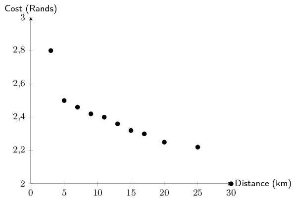
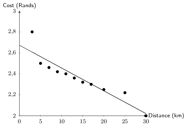
A taxi driver recorded the number of kilometres his taxi travelled per trip and his fuel cost per kilometre in Rands. Examine the table of his data below and answer the questions that follow.

Distance (\(x\))	3	5	7	9	11	13	15	17	20	25	30
Cost (\(y\))	\(\text{2,8}\)	\(\text{2,5}\)	\(\text{2,46}\)	\(\text{2,42}\)	\(\text{2,4}\)	\(\text{2,36}\)	\(\text{2,32}\)	\(\text{2,3}\)	\(\text{2,25}\)	\(\text{2,22}\)	2

Draw a scatter plot of the data.

Use your calculator to determine the equation of the least squares regression line and draw this line on your scatter plot. Round \(a\) and \(b\) to two decimal places in your final answer.

\[\hat{y}=\text{2,67} + -\text{0,02}x\]

Using your calculator, determine the correlation coefficient to two decimal places.

\(r = -\text{0,92}\)

Describe the relationship between the distance travelled per trip and the fuel cost per kilometre.

There is a very strong, negative, linear relationship between distance travelled per trip and the fuel cost per kilometre.

Predict the distance travelled if the cost per kilometre is \(\text{R}\,\text{1,75}\).

\begin{align*} \text{1,75}&=\text{2,67} -\text{0,02}x \\ \therefore x &= \frac{\text{1,75}-\text{2,67}}{-\text{0,02}} = 46 \text{ kilometres} \end{align*}

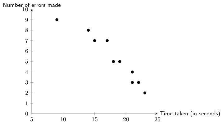
The time taken, in seconds, to complete a task and the number of errors made on the task were recorded for a sample of 10 primary school learners. The data is shown in the table below. [Adapted from NSC Paper 3 Feb-March 2013]

Time taken to complete task (in seconds)	23	21	19	9	15	22	17	14	21	18
Number of errors made	\(\text{2}\)	\(\text{4}\)	\(\text{5}\)	\(\text{9}\)	\(\text{7}\)	\(\text{3}\)	\(\text{7}\)	\(\text{8}\)	\(\text{3}\)	\(\text{5}\)

Draw a scatter plot of the data.

What is the influence of more time taken to complete the task on the number of errors made?

When more time is taken to complete the task, the learners make fewer errors.

When less time is taken to complete the task, the learners make more errors.

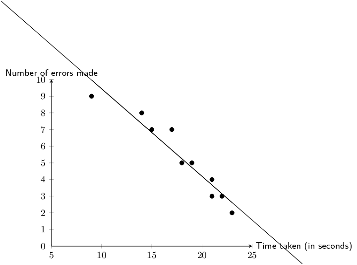
Determine the equation of the least squares regression line and draw this line on your scatter plot. Round \(a\) and \(b\) to two decimal places in your final answer.

\begin{align*} a&= \text{14,71} \\ b&= -\text{0,53} \\ \hat{y}&=\text{14,71} - \text{0,53}x \end{align*}

Determine the correlation coefficient to two decimal places.

\(r = -\text{0,96}\)

Predict the number of errors that will be made by a learner who takes 13 seconds to complete this task.

\begin{align*} \hat{y}&=\text{14,71} -\text{0,53}(13) \\ &\approx \text{7,82} \\ &\approx 8 \end{align*}

Comment on the strength of the relationship between the variables.

There is a strong negative relationship between the variables.

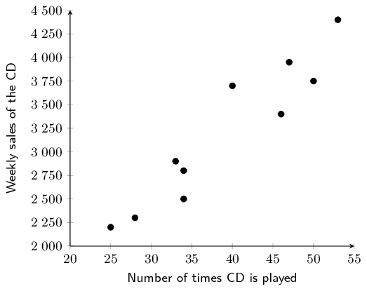
A recording company investigates the relationship between the number of times a CD is played by a national radio station and the national sales of the same CD in the following week. The data below was collected for a random sample of 10 CDs. The sales figures are rounded to the nearest 50. [NSC Paper 3 November 2012]

Number of times CD is played	47	34	40	34	33	50	28	53	25	46
Weekly sales of the CD	\(\text{3 950}\)	\(\text{2 500}\)	\(\text{3 700}\)	\(\text{2 800}\)	\(\text{2 900}\)	\(\text{3 750}\)	\(\text{2 300}\)	\(\text{4 400}\)	\(\text{2 200}\)	\(\text{3 400}\)

Draw a scatter plot of the data.

Determine the equation of the least squares regression line.

\begin{align*} a&=\text{293,06} \\ b&=\text{74,28} \\ \hat{y} &=\text{293,06} + \text{74,28}x \end{align*}

Calculate the correlation coefficient.

\(r=\text{0,95}\)

Predict, correct to the nearest 50, the weekly sales for a CD that was played 45 times by the radio station in the previous week.

\begin{align*} \hat{y}&= \text{293,06} + \text{74,28}(45) \\ &= \text{3 635,66} \\ &\approx \text{3 650} \text{ (to the nearest 50)} \end{align*}

Comment on the strength of the relationship between the variables.

There is a very strong positive relationship between the number of times that a CD was played and the sales of that CD in the following week.

9.2 Curve fitting

Table of Contents

9.4 Summary