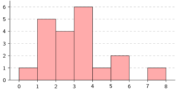
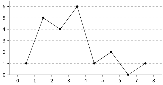
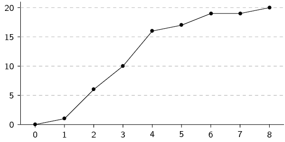
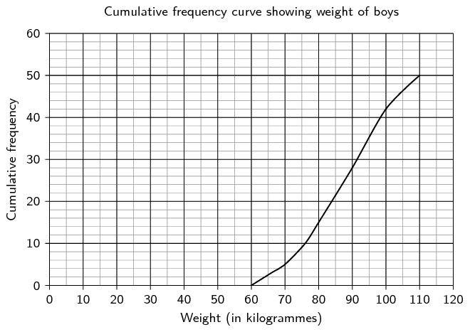
Draw a histogram, frequency polygon and ogive of the following data set.
To count the data, use intervals with a width of \(\text{1}\), starting
from \(\text{0}\).
\(\text{0,4}\) ; \(\text{3,1}\) ; \(\text{1,1}\) ; \(\text{2,8}\) ;
\(\text{1,5}\) ; \(\text{1,3}\) ; \(\text{2,8}\) ; \(\text{3,1}\) ;
\(\text{1,8}\) ; \(\text{1,3}\) ;
\(\text{2,6}\) ; \(\text{3,7}\) ; \(\text{3,3}\) ; \(\text{5,7}\) ;
\(\text{3,7}\) ; \(\text{7,4}\) ; \(\text{4,6}\) ; \(\text{2,4}\) ;
\(\text{3,5}\) ; \(\text{5,3}\)
We first organise the data into a table using an interval width of
\(\text{1}\), showing the count in each interval as well as the
cumulative count across intervals.
| Interval |
\([\text{0};\text{1})\) |
\([\text{1};\text{2})\) |
\([\text{2};\text{3})\) |
\([\text{3};\text{4})\) |
\([\text{4};\text{5})\) |
\([\text{5};\text{6})\) |
\([\text{6};\text{7})\) |
\([\text{7};\text{8})\) |
| Count |
\(\text{1}\) |
\(\text{5}\) |
\(\text{4}\) |
\(\text{6}\) |
\(\text{1}\) |
\(\text{2}\) |
\(\text{0}\) |
\(\text{1}\) |
| Cumulative |
\(\text{1}\) |
\(\text{6}\) |
\(\text{10}\) |
\(\text{16}\) |
\(\text{17}\) |
\(\text{19}\) |
\(\text{19}\) |
\(\text{20}\) |
From the table above we can draw the histogram, frequency polygon and ogive.


Draw a box and whisker diagram of the following data set and explain whether
it is symmetric, skewed right or skewed left.
\(-\text{4,1}\) ; \(-\text{1,1}\) ; \(-\text{1}\) ; \(-\text{1,2}\) ;
\(-\text{1,5}\) ; \(-\text{3,2}\) ; \(-\text{4}\) ; \(-\text{1,9}\) ;
\(-\text{4}\) ;
\(-\text{0,8}\) ; \(-\text{3,3}\) ; \(-\text{4,5}\) ; \(-\text{2,5}\) ;
\(-\text{4,4}\) ; \(-\text{4,6}\) ; \(-\text{4,4}\) ; \(-\text{3,3}\)
The statistics of the data set are
- minimum: \(-\text{4,6}\);
- first quartile: \(-\text{4,1}\);
- median: \(-\text{3,3}\);
- third quartile: \(-\text{1,5}\);
- maximum: \(-\text{0,8}\).
From this we can draw the box-and-whisker plot as follows.

Since the median is closer to the first quartile than the third quartile, the
data set is skewed right.
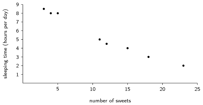
What is the mean and standard deviation of the number of
sweets eaten per day?
Mean = \(11 \frac{3}{8}\). Standard deviation =
\(\text{6,69}\).
What is the mean and standard deviation of the number of
hours slept per day?
Mean = \(5 \frac{3}{8}\). Standard deviation =
\(\text{2,33}\).
Make a list of all the outliers in the data set.
There are no outliers.
What is the mean and standard deviation of their incomes?
Mean = \(\text{R}\,\text{12 497,50}\). Standard deviation
= \(\text{R}\,\text{1 768,55}\).
How many of the salaries are less than one standard
deviation away from the mean?
All salaries within the range \((\text{10 728,95}\ ;\
\text{14 266,05})\) are less than one standard deviation
away from the mean.
There are \(\text{4}\) salaries inside this range.
If each teacher gets a bonus of \(\text{R}\,\text{500}\) added to
their pay what is the new mean and standard deviation?
Since the increase in each salary is the same absolute amount, the
mean simply increases by the bonus.
The standard deviation does not change since every value is
increased by exactly the same amount.
Mean = \(\text{R}\,\text{12 997,50}\). Standard deviation =
\(\text{R}\,\text{1 768,55}\).
If each teacher gets a bonus of \(\text{10}\%\) on their salary what
is the new mean and standard deviation?
With a relative increase, the mean and standard deviation are both
multiplied by the same factor.
With an increase of \(\text{10}\%\) the factor is
\(\text{1,1}\).
Mean = \(\text{R}\,\text{13 747,25}\). Standard deviation =
\(\text{R}\,\text{1 945,41}\).
Determine for both of the above, how many salaries are less
than one standard deviation away from the mean.
Adding a constant amount or multiplying by a constant factor (that
is, applying a linear transformation) does not change the number
of values that lie within one standard deviation from the mean.
Therefore the answer is still \(\text{4}\).
Using the above information work out which bonus is more
beneficial financially for the teachers.
Since the mean is greater in the second case it means that, on
average, the teachers are getting better salaries when the
increase is \(\text{10}\%\).
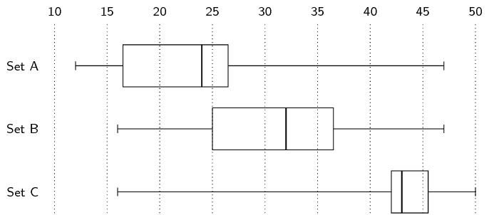
For each of the sets calculate the mean and the five number
summary.
A. Mean = \(\text{23,83}\). Five number summary = [ \(\text{12}\) ;
\(\text{16,5}\) ; \(\text{24}\) ; \(\text{26,5}\) ;
\(\text{47}\) ].
B. Mean = \(\text{31,17}\). Five number summary = [ \(\text{16}\) ;
\(\text{25}\) ; \(\text{32}\) ; \(\text{36,5}\) ; \(\text{47}\)
].
C. Mean = \(\text{41,83}\). Five number summary = [ \(\text{16}\) ;
\(\text{42}\) ; \(\text{43}\) ; \(\text{45,5}\) ; \(\text{50}\)
].
Make box and whisker plots of the three data sets on the
same set of axes.
State, with reasons, whether each of the three data sets
are symmetric or skewed (either right or left).
Set A: skewed left. Set B: slightly skewed left. Set C:
skewed right.
