Home Practice
For learners and parents For teachers and schools
Textbooks
Full catalogue
Leaderboards
Learners Leaderboard Classes/Grades Leaderboard Schools Leaderboard
Pricing Support
Help centre Contact us
Log in

We think you are located in United States. Is this correct?

14.2 Relative frequency

14.2 Relative frequency (EMA7X)

temp text
Relative frequency

The relative frequency of an event is defined as the number of times that the event occurs during experimental trials, divided by the total number of trials conducted.

The relative frequency is not a theoretical quantity, but an experimental one. We have to repeat an experiment a number of times and count how many times the outcome of the trial is in the event set. Because it is experimental, it is possible to get a different relative frequency every time that we repeat an experiment.

The following video explains the concept of relative frequency using the throw of a dice.

Video: 2GW7

temp text

Worked example 2: Relative frequency and theoretical probability

We toss a coin \(\text{30}\) times and observe the outcomes. The results of the trials are shown in the table below.

trial

\(\text{1}\)

\(\text{2}\)

\(\text{3}\)

\(\text{4}\)

\(\text{5}\)

\(\text{6}\)

\(\text{7}\)

\(\text{8}\)

\(\text{9}\)

\(\text{10}\)

outcome

H

T

T

T

H

T

H

H

H

T

trial

\(\text{11}\)

\(\text{12}\)

\(\text{13}\)

\(\text{14}\)

\(\text{15}\)

\(\text{16}\)

\(\text{17}\)

\(\text{18}\)

\(\text{19}\)

\(\text{20}\)

outcome

H

T

T

H

T

T

T

H

T

T

trial

\(\text{21}\)

\(\text{22}\)

\(\text{23}\)

\(\text{24}\)

\(\text{25}\)

\(\text{26}\)

\(\text{27}\)

\(\text{28}\)

\(\text{29}\)

\(\text{30}\)

outcome

H

H

H

T

H

T

H

T

T

T

What is the relative frequency of observing heads after each trial and how does it compare to the theoretical probability of observing heads?

Count the number of positive outcomes

A positive outcome is when the outcome is in our event set. The table below shows a running count (after each trial \(t\)) of the number of positive outcomes \(p\) we have observed. For example, after \(t = 20\) trials we have observed heads \(\text{8}\) times and tails \(\text{12}\) times and so the positive outcome count is \(p = 8\).

\(t\)

\(\text{1}\)

\(\text{2}\)

\(\text{3}\)

\(\text{4}\)

\(\text{5}\)

\(\text{6}\)

\(\text{7}\)

\(\text{8}\)

\(\text{9}\)

\(\text{10}\)

\(p\)

\(\text{1}\)

\(\text{1}\)

\(\text{1}\)

\(\text{1}\)

\(\text{2}\)

\(\text{2}\)

\(\text{3}\)

\(\text{4}\)

\(\text{5}\)

\(\text{5}\)

\(t\)

\(\text{11}\)

\(\text{12}\)

\(\text{13}\)

\(\text{14}\)

\(\text{15}\)

\(\text{16}\)

\(\text{17}\)

\(\text{18}\)

\(\text{19}\)

\(\text{20}\)

\(p\)

\(\text{6}\)

\(\text{6}\)

\(\text{6}\)

\(\text{7}\)

\(\text{7}\)

\(\text{7}\)

\(\text{7}\)

\(\text{8}\)

\(\text{8}\)

\(\text{8}\)

\(t\)

\(\text{21}\)

\(\text{22}\)

\(\text{23}\)

\(\text{24}\)

\(\text{25}\)

\(\text{26}\)

\(\text{27}\)

\(\text{28}\)

\(\text{29}\)

\(\text{30}\)

\(p\)

\(\text{9}\)

\(\text{10}\)

\(\text{11}\)

\(\text{11}\)

\(\text{12}\)

\(\text{12}\)

\(\text{13}\)

\(\text{13}\)

\(\text{13}\)

\(\text{13}\)

Compute the relative frequency

Since the relative frequency is defined as the ratio between the number of positive trials and the total number of trials,

\[f=\frac{p}{t}\]

The relative frequency of observing heads, \(f\), after having completed \(t\) coin tosses is:

\(t\)

\(\text{1}\)

\(\text{2}\)

\(\text{3}\)

\(\text{4}\)

\(\text{5}\)

\(\text{6}\)

\(\text{7}\)

\(\text{8}\)

\(\text{9}\)

\(\text{10}\)

\(f\)

\(\text{1,00}\)

\(\text{0,50}\)

\(\text{0,33}\)

\(\text{0,25}\)

\(\text{0,40}\)

\(\text{0,33}\)

\(\text{0,43}\)

\(\text{0,50}\)

\(\text{0,56}\)

\(\text{0,50}\)

\(t\)

\(\text{11}\)

\(\text{12}\)

\(\text{13}\)

\(\text{14}\)

\(\text{15}\)

\(\text{16}\)

\(\text{17}\)

\(\text{18}\)

\(\text{19}\)

\(\text{20}\)

\(f\)

\(\text{0,55}\)

\(\text{0,50}\)

\(\text{0,46}\)

\(\text{0,50}\)

\(\text{0,47}\)

\(\text{0,44}\)

\(\text{0,41}\)

\(\text{0,44}\)

\(\text{0,42}\)

\(\text{0,40}\)

\(t\)

\(\text{21}\)

\(\text{22}\)

\(\text{23}\)

\(\text{24}\)

\(\text{25}\)

\(\text{26}\)

\(\text{27}\)

\(\text{28}\)

\(\text{29}\)

\(\text{30}\)

\(f\)

\(\text{0,43}\)

\(\text{0,45}\)

\(\text{0,48}\)

\(\text{0,46}\)

\(\text{0,48}\)

\(\text{0,46}\)

\(\text{0,48}\)

\(\text{0,46}\)

\(\text{0,45}\)

\(\text{0,43}\)

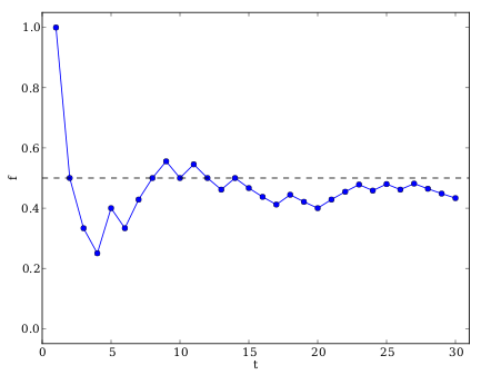
From the last entry in this table we can now easily read the relative frequency after \(\text{30}\) trials, namely \(\frac{13}{30} = \text{0,4}\dot{3}\). The relative frequency is close to the theoretical probability of \(\text{0,5}\). In general, the relative frequency of an event tends to get closer to the theoretical probability of the event as we perform more trials.

A much better way to summarise the table of relative frequencies is in a graph:

The graph above is the plot of the relative frequency of observing heads, \(f\), after having completed \(t\) coin tosses. It was generated from the table of numbers above by plotting the number of trials that have been completed, \(t\), on the \(x\)-axis and the relative frequency, \(f\), on the \(y\)-axis. In the beginning (after a small number of trials) the relative frequency fluctuates a lot around the theoretical probability at \(\text{0,5}\), which is shown with a dashed line. As the number of trials increases, the relative frequency fluctuates less and gets closer to the theoretical probability.

Worked example 3: Relative frequency and theoretical probability

While watching \(\text{10}\) soccer games where Team 1 plays against Team 2, we record the following final scores:

Trial

\(\text{1}\)

\(\text{2}\)

\(\text{3}\)

\(\text{4}\)

\(\text{5}\)

\(\text{6}\)

\(\text{7}\)

\(\text{8}\)

\(\text{9}\)

\(\text{10}\)

Team 1

\(\text{2}\)

\(\text{0}\)

\(\text{1}\)

\(\text{1}\)

\(\text{1}\)

\(\text{1}\)

\(\text{1}\)

\(\text{0}\)

\(\text{5}\)

\(\text{3}\)

Team 2

\(\text{0}\)

\(\text{2}\)

\(\text{2}\)

\(\text{2}\)

\(\text{2}\)

\(\text{1}\)

\(\text{1}\)

\(\text{0}\)

\(\text{0}\)

\(\text{0}\)

What is the relative frequency of Team 1 winning?

In this experiment, each trial takes the form of Team 1 playing a soccer match against Team 2.

Count the number of positive outcomes

We are interested in the event where Team 1 wins. From the table above we see that this happens \(\text{3}\) times.

Compute the relative frequency

The total number of trials is \(\text{10}\). This means that the relative frequency of the event is

\[\frac{3}{10} = \text{0,3}\]

It is important to understand the difference between the theoretical probability of an event and the observed relative frequency of the event in experimental trials. The theoretical probability is a number that we can compute if we have enough information about the experiment. If each possible outcome in the sample space is equally likely, we can count the number of outcomes in the event set and the number of outcomes in the sample space to compute the theoretical probability.

The relative frequency depends on the sequence of outcomes that we observe while doing a statistical experiment. The relative frequency can be different every time we redo the experiment. The more trials we run during an experiment, the closer the observed relative frequency of an event will get to the theoretical probability of the event.

So why do we need statistical experiments if we have theoretical probabilities? In some cases, like our soccer experiment, it is difficult or impossible to compute the theoretical probability of an event. Since we do not know exactly how likely it is that one soccer team will score goals against another, we can never compute the theoretical probability of events in soccer. In such cases we can still use the relative frequency to estimate the theoretical probability, by running experiments and counting the number of positive outcomes.

You can use this Phet simulation on probability to do some experiments with dropping a ball through a triangular grid.

Textbook Exercise 14.2

A die is tossed 44 times and lands 5 times on the number 3.

What is the relative frequency of observing the die land on the number 3? Write your answer correct to 2 decimal places.

Recall the formula: \[f = \frac{p}{t}\]

Identify variables needed: \begin{align*} p & = \text{number of positive trials} = \text{5} \\ f & = \text{total number of trials} = \text{44} \end{align*}

Calculate the relative frequency: \begin{align*} f & = \frac{p}{t} \\ & = \frac{\text{5}}{\text{44}} \\ & = \text{0,11} \end{align*}

Therefore, the relative frequency of observing the die on the number 3 is \(\text{0,11}\).

A coin is tossed 30 times and lands 17 times on heads.

What is the relative frequency of observing the coin land on heads? Write your answer correct to 2 decimal places.

Recall the formula: \[f = \frac{p}{t}\]

Identify variables needed: \begin{align*} p & = \text{number of positive trials} = \text{17} \\ f & = \text{total number of trials} = \text{30} \end{align*}

Calculate the relative frequency: \begin{align*} f & = \frac{p}{t} \\ & = \frac{\text{17}}{\text{30}} \\ & = \text{0,57} \end{align*}

Therefore, the relative frequency of observing the coin on heads is \(\text{0,57}\).

A die is tossed 27 times and lands 6 times on the number 6.

What is the relative frequency of observing the die land on the number 6? Write your answer correct to 2 decimal places.

Recall the formula: \[f = \frac{p}{t}\]

Identify variables needed: \begin{align*} p & = \text{number of positive trials} = \text{6} \\ f & = \text{total number of trials} = \text{27} \end{align*}

Calculate the relative frequency: \begin{align*} f & = \frac{p}{t} \\ & = \frac{\text{6}}{\text{27}} \\ & = \text{0,22} \end{align*}

Therefore, the relative frequency of observing the die on the number 6 is \(\text{0,22}\).