12.5 Classifying and organising data
|
Previous
12.4 Collecting data
|
Next
12.6 Summarising data
|
12.5 Classifying and organising data (EMG6Z)
Classifying data (EMG72)
After data has been collected, the next stage in the data handling process is to classify it. There are two main ways data can be classified. These are:
-
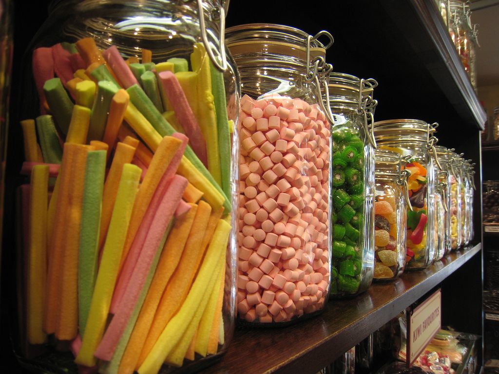
Categorical data: This is data that cannot be measured numerically but can be described, like the gender of a person (male or female), or the colours of sweets in a jar.

-
Numerical data: This is data that can be measured by using numbers, like the height of person or the number of books in your bag.

Numerical data can be further classified into discrete data and continuous data. Data is discrete if each value can only have one specific value that can be counted. Examples of discrete data would be a number of bicycles (\(\text{1}\); \(\text{5}\); \(\text{8}\), not \(\frac{\text{1}}{\text{2}}\) a bicycle!) or the number of puppies in a litter (again: \(\text{3}\) puppies; \(\text{6}\) puppies but not \(\frac{\text{1}}{\text{3}}\) of a puppy!)
Continuous data is data that can have any value - for example, a person's weight may be anything between \(\text{50}\) or \(\text{100}\) \(\text{kg}\), including \(\text{67,4}\) \(\text{kg}\) or \(\text{78,3}\) \(\text{kg}\). Weight is not only measured in single kilograms. The amount of rainfall is also continuous data - it can be any amount and is not limited to specific kinds of values (rain does not only fall in \(\text{100}\) \(\text{ml}\) quantities, for example!).
Organising data (EMG73)
Data can be organised by using :
-
Tallies - Tallies are a way of counting how many of each group there are. The advantage of using tallies is that you can keep a running total.
Here is an example of a tally table showing numbers of differently coloured cars (Note that each counted item is represented by one line marking):
Car colours
Colour
Tally
Red


Green

Blue

Yellow

For each differently coloured car we see, we make a mark. When we get to \(\text{5}\) cars, we draw a line through the previous four marks and then start a new group of marks. This makes it easy to count up the tallies in groups of \(\text{5}\) markings.
- Frequency tables - A frequency table shows the list of categories or groups of things, together with the number of times the items occur. Here is an example of a frequency table, again, showing the number of differently coloured cars. The frequency is the same as the number of marks we made in the tally table above. Car colours
Colour | Frequency |
Red | \(\text{7}\) |
Green | \(\text{3}\) |
Blue | \(\text{4}\) |
Yellow | \(\text{2}\) |
- Class intervals - when you have a lot of data to organise, e.g. heights of \(\text{15}\) year old learners in a school, it becomes easier to manage if these heights are grouped into specific bands. Here is an example of grouped data showing the heights of \(\text{32}\) Grade 10 learners.
Height range | Number of learners (Frequency) |
\( | \(\text{1}\) |
\(\text{1,20}\) \(\text{m}\) - \(\text{1,29}\) \(\text{m}\) | \(\text{0}\) |
\(\text{1,30}\) \(\text{m}\) - \(\text{1,39}\) \(\text{m}\) | \(\text{2}\) |
\(\text{1,40}\) \(\text{m}\) - \(\text{1,49}\) \(\text{m}\) | \(\text{4}\) |
\(\text{1,50}\) \(\text{m}\) - \(\text{1,59}\) \(\text{m}\) | \(\text{7}\) |
\(\text{1,60}\) \(\text{m}\) - \(\text{1,69}\) \(\text{m}\) | \(\text{11}\) |
\(\text{1,79}\) \(\text{m}\) - \(\text{1,79}\) \(\text{m}\) | \(\text{7}\) |
\(>\) \(\text{1,80}\) \(\text{m}\) | \(\text{0}\) |
|
Previous
12.4 Collecting data
|
Table of Contents |
Next
12.6 Summarising data
|
